Objectives

• Simulate lowpass, highpass, and bandpass filters on LTSpice
• Build a basic microphone circuit and test it with MATLAB and the Nano Every
• Build an amplifier circuit and test it with MATLAB and the Nano Every
• Implement a filter, characterize it, and compare its frequency response to the simulated response on LTSpice
• Test the entire circuit only using the Ardunio Nano Every
• Charactize your circuita and adapt the code for the final demonstration

Materials

• Robot
• Various capacitors and resistors
• 1x LM358 op-amp
• 1x microphone
• LTSpice
• MATLAB

Simulating Filters in LTSpice

The goal for this part of the lab was to get familiar with LTSpice by simulating a lowpass and highpass filter with a cutoff frequency around 1.3kHz with a resistor value of 1.2kΩ and a capacitor value of .1µF. We then plotted the transfer function of each filter, which is shown below.

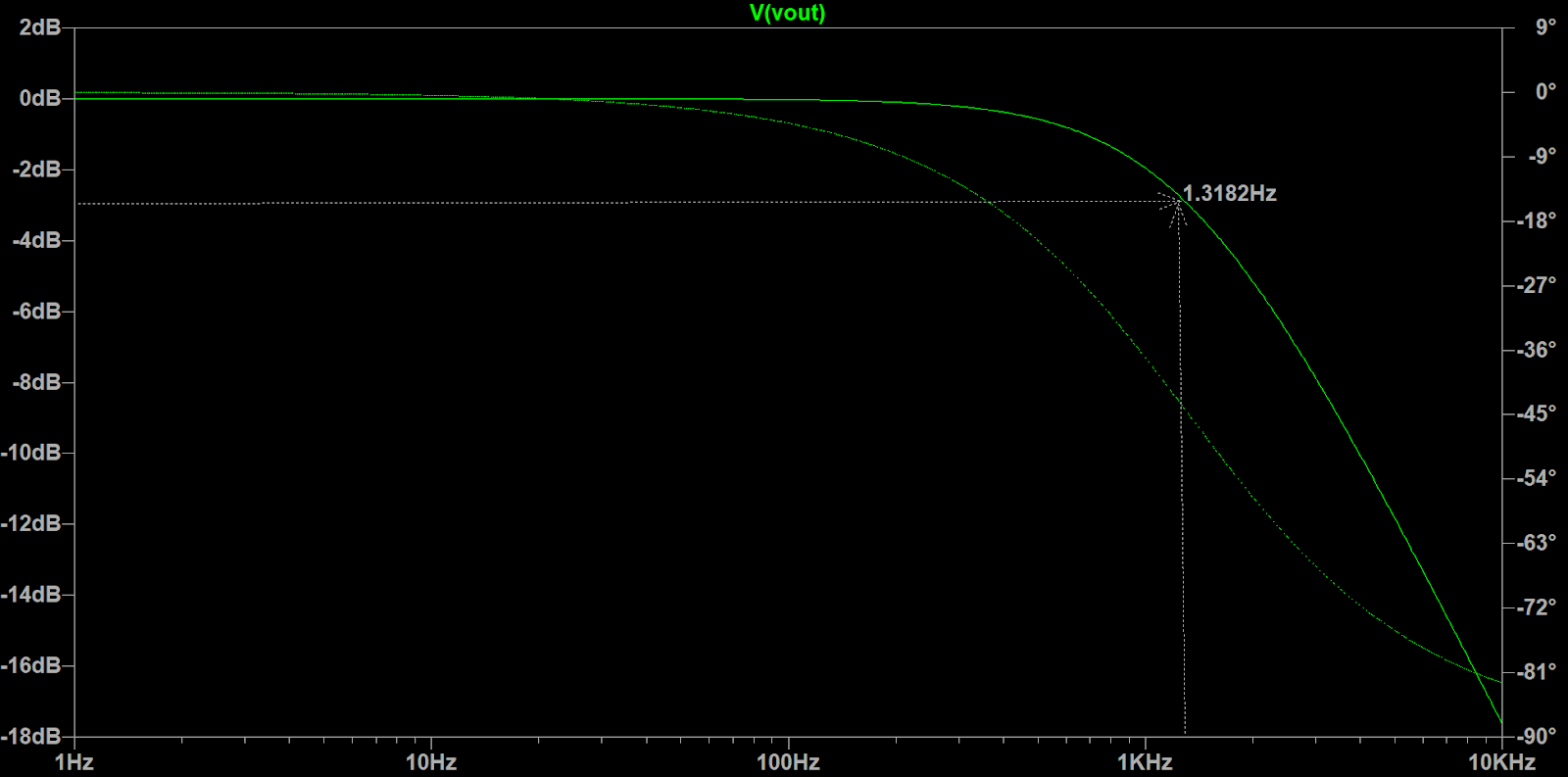
Above is a screenshot of the lowpass filter simulated on LTSpice.

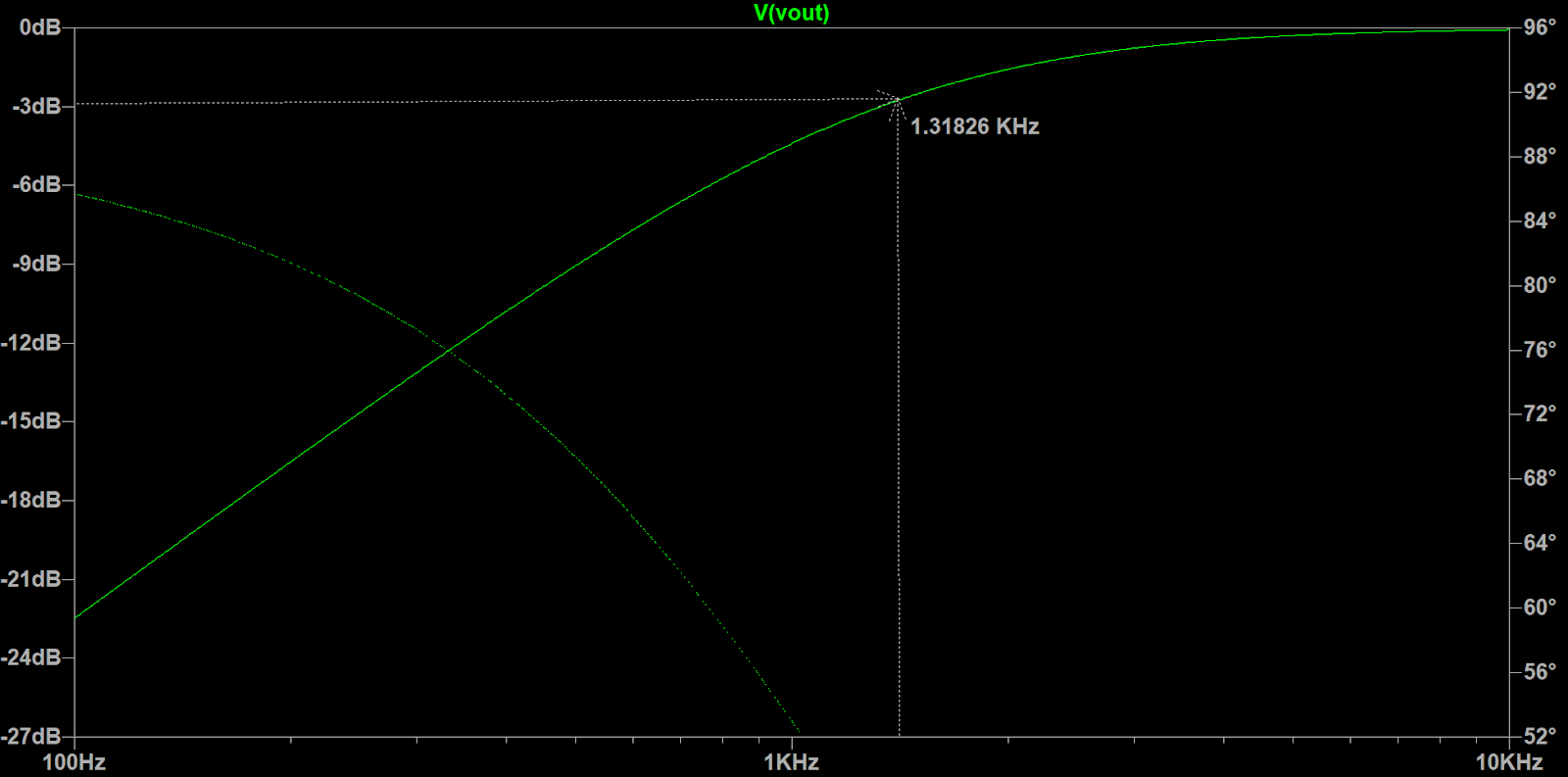
Above is a screenshot of the highpass filter simulated on LTSpice.

Building and Testing Basic Microphone Circuit

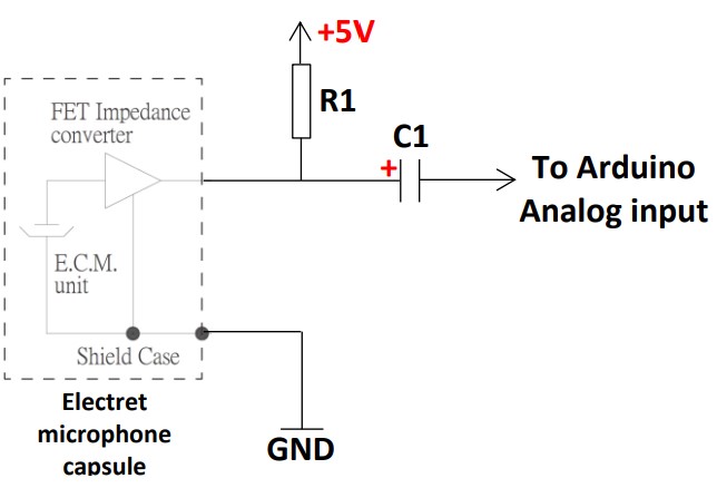
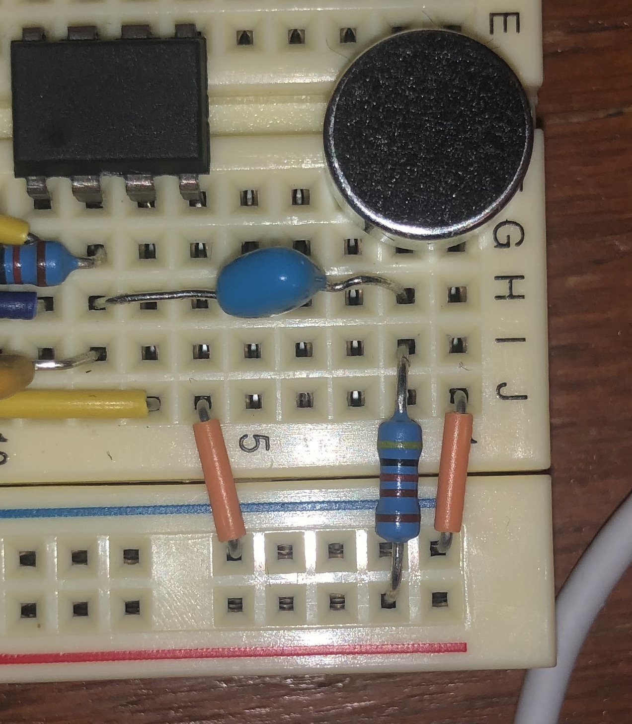
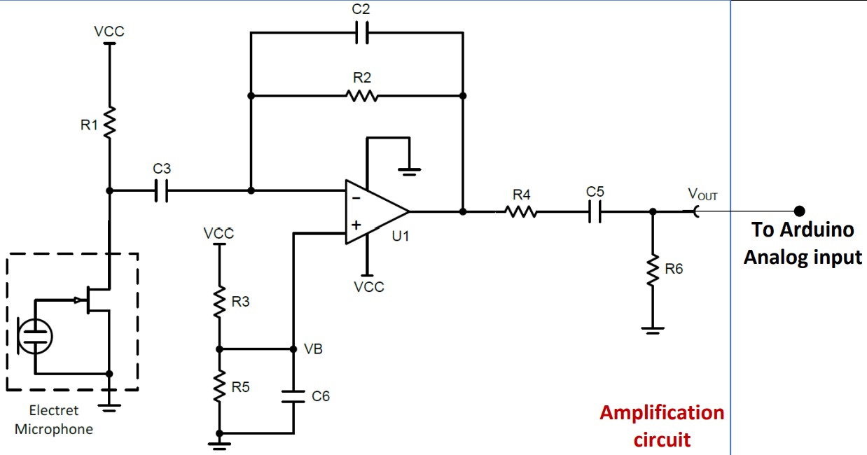
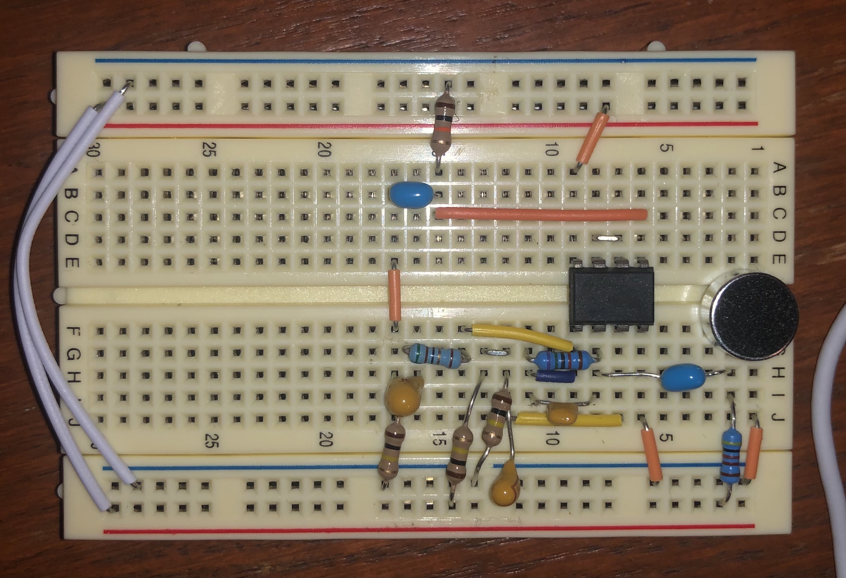
For the final demo, we will need to be able to start when a certain sound of a given frequency. To do this, we will use a microphone. Below is a diagram of the microphone circuit that we will build, followed by a picture of the microphone circuit itself.

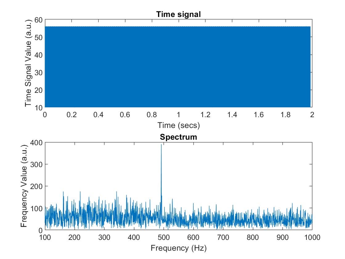
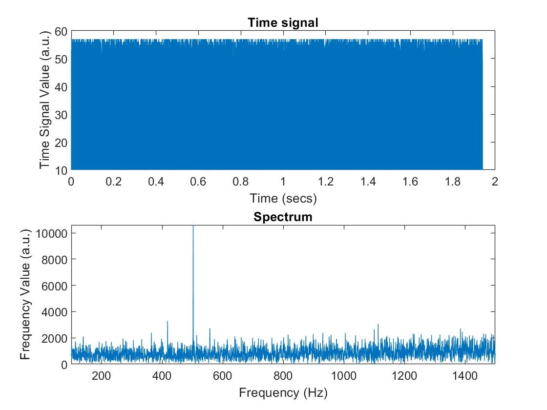
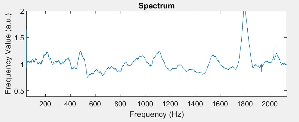
To test if the microphone is working properly, we manually coded the ADC in free-running mode to convert the analog signal from the microphone circuit to a digital one so that we can visualize the data. From here, we used MATLAB to collect and analyze the data with Fourier Analysis. When a sound of a certain frequency is played, MATLAB performs the analysis and displays the data. For example, when 500 Hz is played, a sharp peak occurs at the respective frequency, as in the graph below, which proves our circuit is properly working.

Building Amplifier Circuit

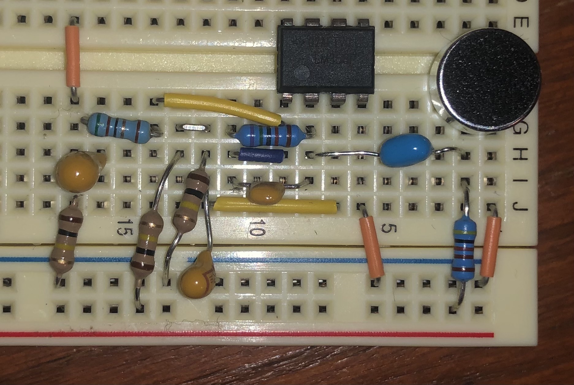
Although the microphone is working properly, it will not be able to distinguish frequencies being played unless it is inches away from the circuit. We want it to pick up sounds from a sizable distance away. To resolve this issue, we will build an amplifier to amplify the analog output from the microphone. Below is a diagram of the amplifier circuit that we will build, followed by a picture of the amplifier circuit itself.

We tested the new amplifier circuit the same way as we tested the simple microphone circuit. As shown below, the amplifier works as intended by significantly increasing the magnitude at all the frequencies, especially the more prominent ones, 500 Hz in this case.

Building and Testing Amplified Circuit with Filter

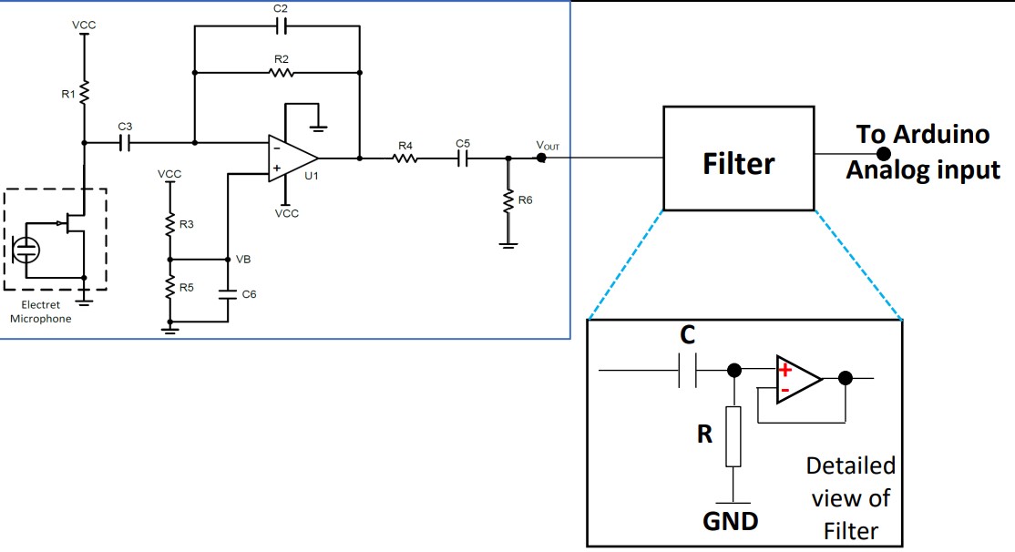
Although a filter is not a necessary component of the final demo, we wanted to apply our knowledge and actually build one ourselves. So, we built a high pass filter with a cutoff around 750 Hz by using capacitor and resistor values of .022µF and 10kHz respectively. Below is a diagram of the amplifier circuit with the high pass filter that we will build, followed by a picture of the circuit itself.

Now to test the filter, we want to plot the transfer function of the experimental high pass filter, the one built on our robot, to that of a simulated circuit on LTSpice. To get the transfer function of the experimental filter, we played a sound that sweeped from 100 Hz to 2000 Hz, and then collected data from the input and output of the filter. When we collected the data, we made sure to keep the microphone at the same distance so that the conditions of both takes were as similar as possible. Now with the data of the input and output, we smoothed data sets to eliminate instances of noise which is common with a USB connection, and then we simply divided the output by the input to get the transfer function. Below is our graph of the experimental transfer function, followed by the simulated transfer function.

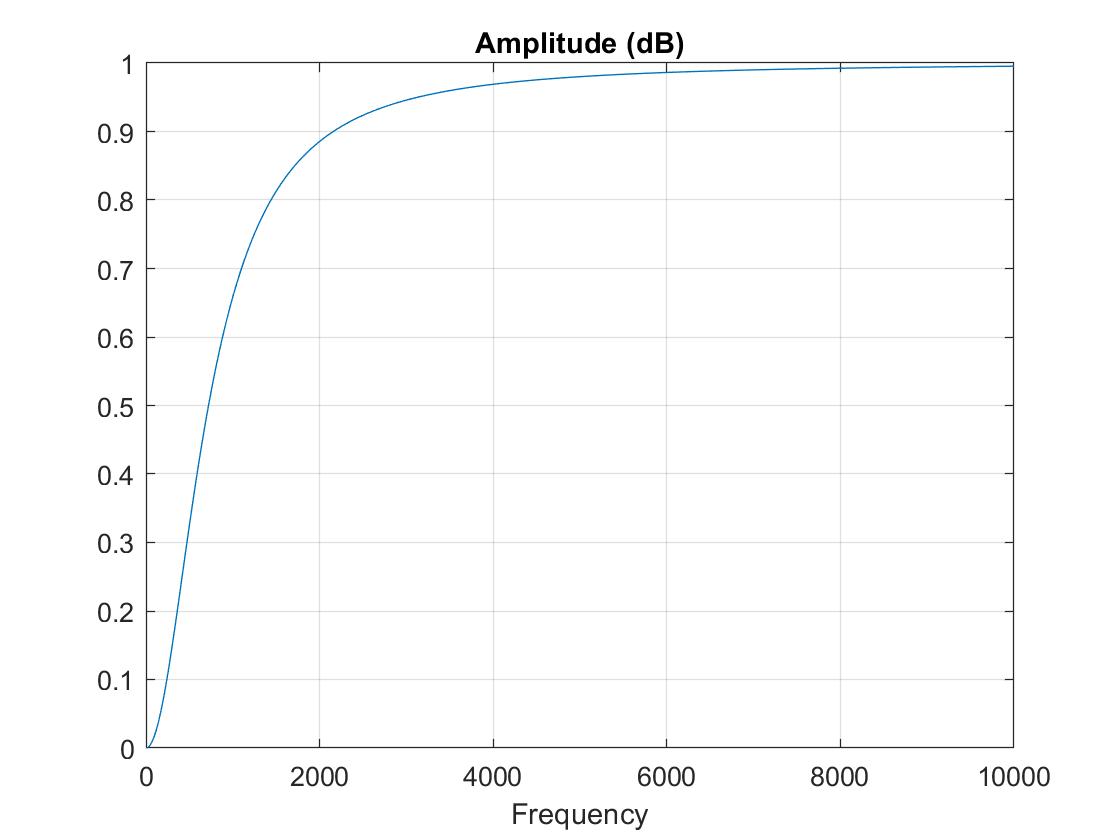
The graph of the transfer function appears to have a cutoff at around 750 Hz, with lower frequencies being killed and higher frequencies passing through normally. However, the experimental graph is different from the simulated graph. This could be attributed to noise from the USB cable or other components of the circuit. Additionally, I personally built this circuit twice with all new components because the transfer function resulting from the first circuit was not at all as expected. The second time around, the transfer function was only slightly more clear. In both cases, multiple TAs verified the circuit was wired correctly, so it leads me to believe that some components were inherently faulty.

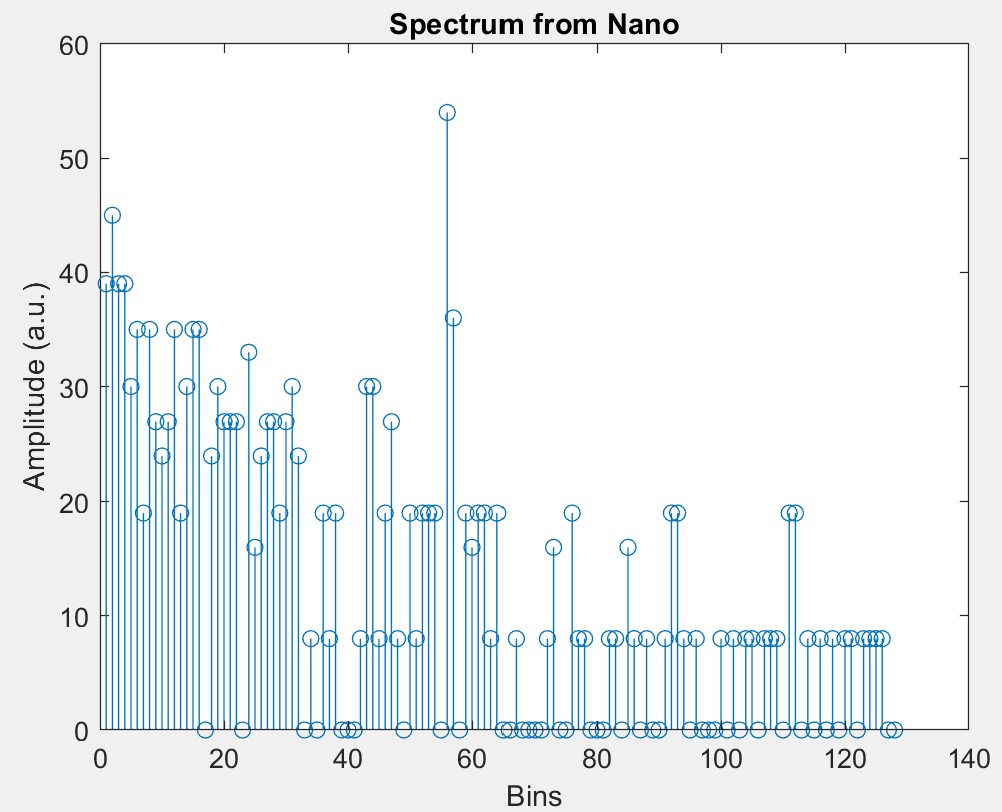
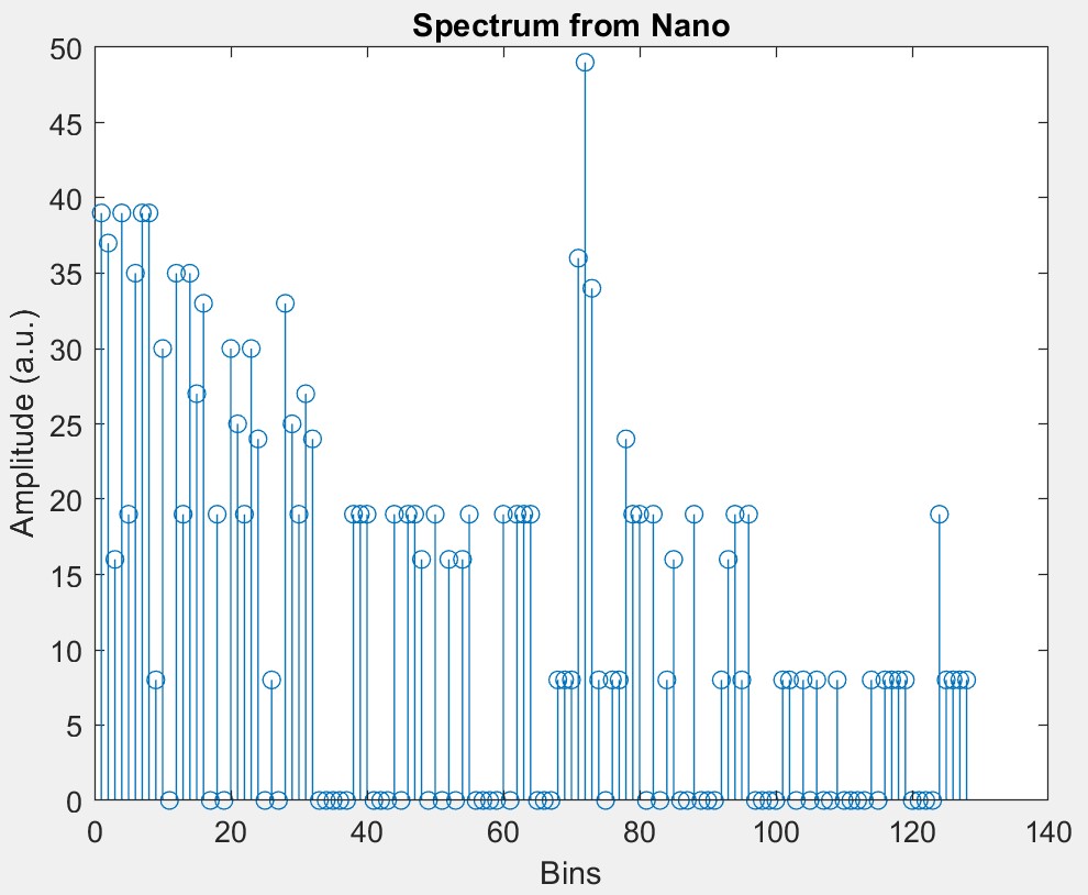
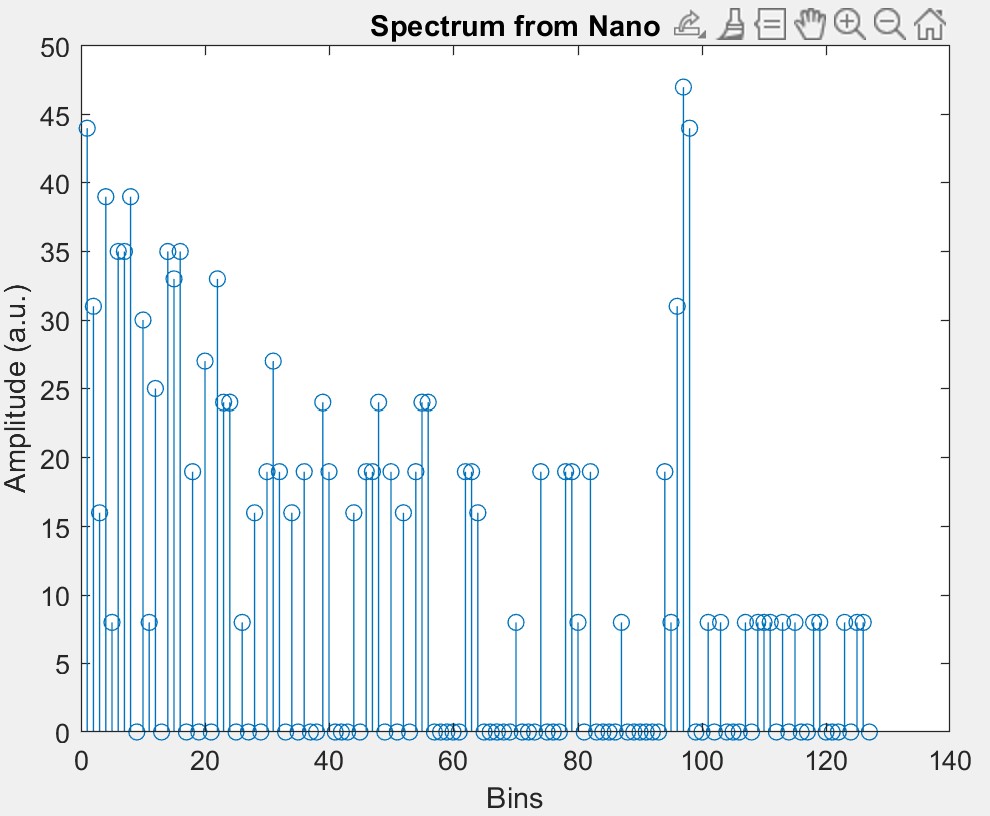
Performing FFT Exclusively on Arduino

Although using MATLAB to perform the analysis of the inputted signal works well when attached with a USB cable, for the final demo, we want to perform all the analysis strictly on the Arduino. To do this, we used a FFT library that will do the analysis for us. Before this could happen though, we need to slow down the ADC to only take values at an interval of .41667ms, which was done by manipulating the TCA with interrupts. With this done, we used a for loop to store the ADC values into an array from which the FFT library’s functions would perform the analysis on. We then printed the values of the FFT to the serial monitor where then copied them into MATLAB to visualize. The graphs of 500 Hz, 700 Hz, and 900 Hz are displayed below, respectively.

Gallery