Summary
In lab 3, we built a basic microphone circuit, an amplifier circuit, and a high pass filter in order to reliably detect the frequency of tones played near the mic, which we'll need to start our final demo in response to a tone. We also simulated a high-pass and low-pass filter in LTSpice and conducted fast Fourier transforms (FFTs) both in Matlab and on the Arduino itself to isolate the most prominent frequencies.
Part 1: Low-Pass and High-Pass Filters in LTSpice
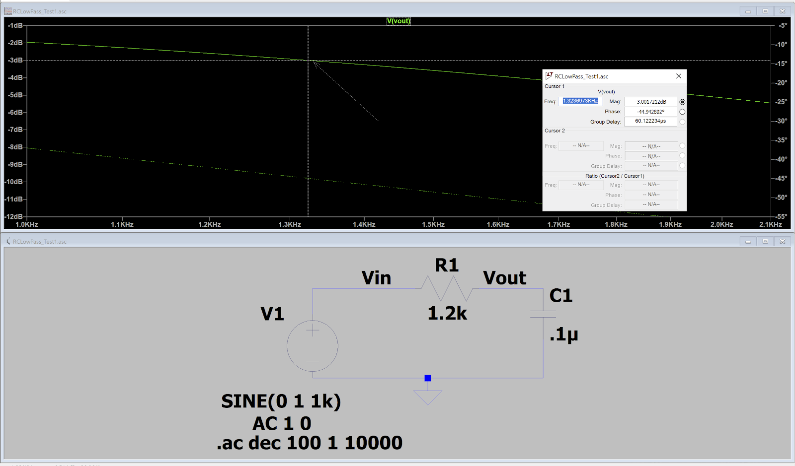
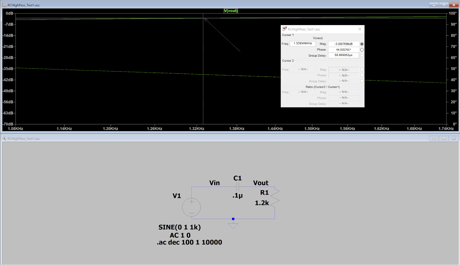
To distinguish between low-pass and high-pass filters and observe the expected behavior of the high-pass filter we would later build, we simulated two filters in LTSpice using given resistor and capacitor values. The simulated circuit and Bode plots are shown below, with low-pass on the left and high-pass on the right. Because both filters used the same resistor and capacitor values, they both had cutoff frequencies of about 1.3 kHz. The difference was in the order of components and whether high or low frequencies were allowed to pass through the filter.
Part 2: Microphone Circuits
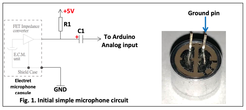
Next, we built a basic microphone circuit, added an amplifier, and characterized the circuits using Matlab. The schematic for the basic microphone circuit is shown below.
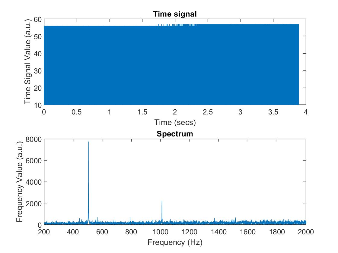
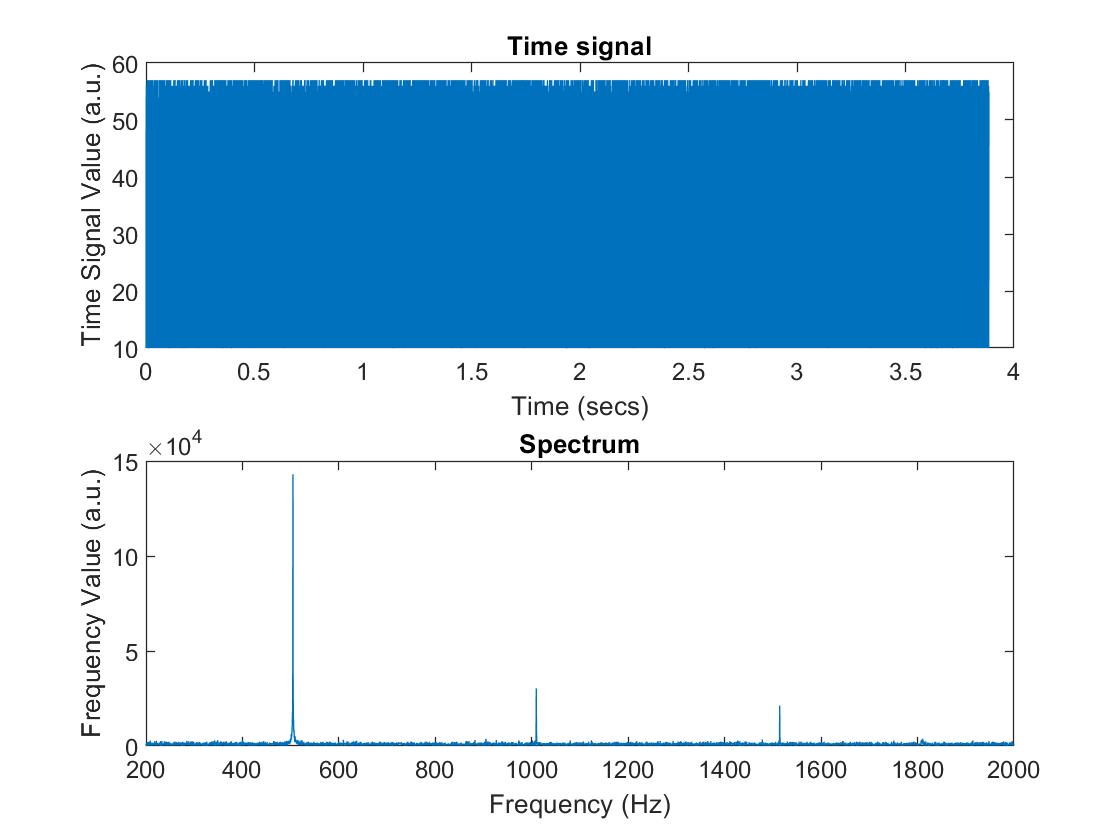
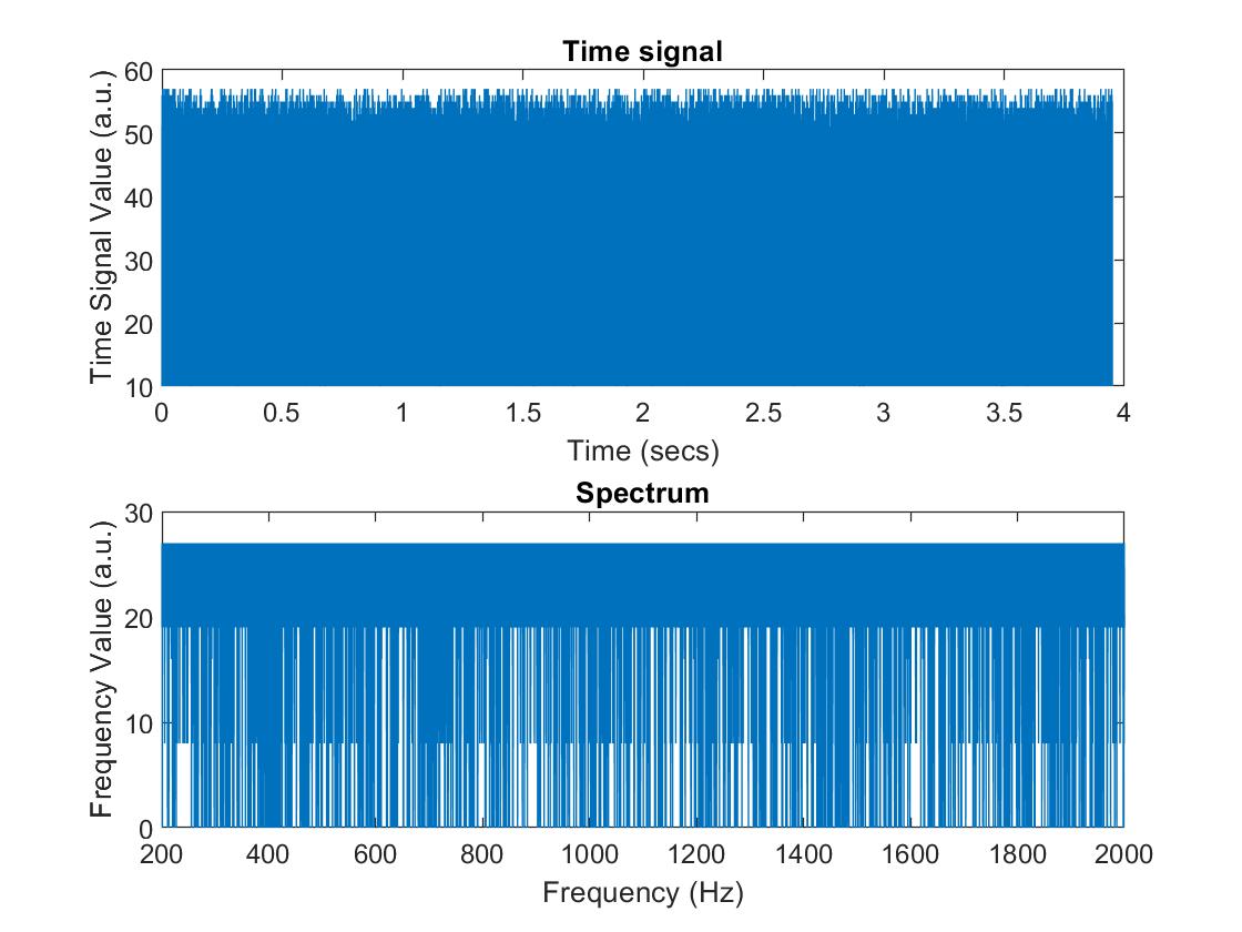
Once the circuit was built, we coded the Arduino to collect sound using the analog to digital (ADC) converter and print it to the serial port. To do this, we enabled the ADC in free-running mode and had the Arduino continuously read in values. Then, we coded a Matlab script to play a tone or range of tones of specified frequencies, collect a specified number of values based on the baud rate from the Ardino, store the Ardunio data as a function of time, and take the FFT of the data. The Matlab script then plotted signal vs. time and the FFT spectrum vs. frequency. The results of playing a 500 Hz tone near our initial unamplified microphone circuit are plotted below.
Next, we amplified the microphone output going into the ADC on the Arduino by building an amplifier circuit, a schematic of which is shown below.
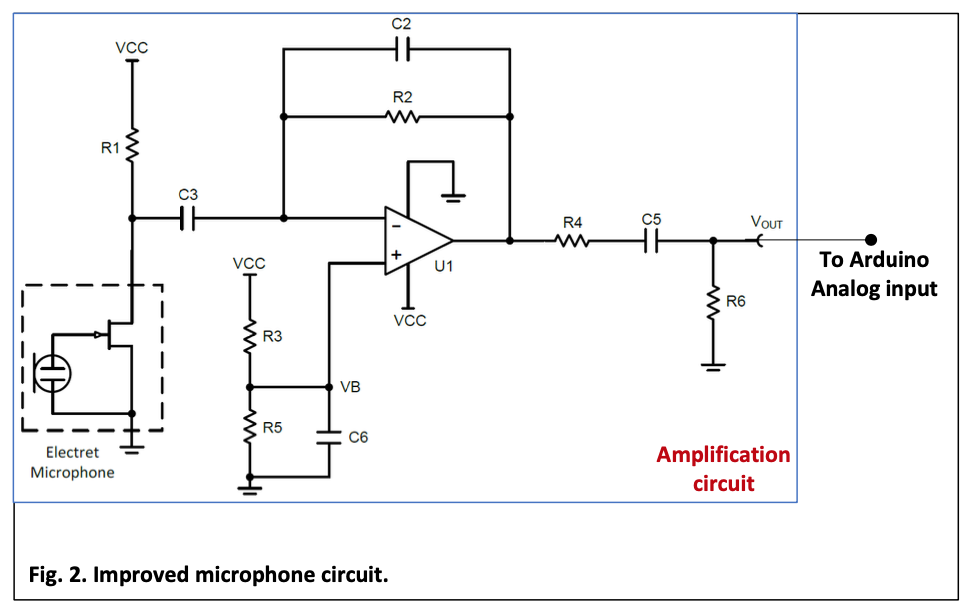
When the 500 Hz signal was amplified, the noise almost disappeared, as demonstrated by the high amplitude at 500 Hz on the Fourier transform graph.
Part 3: High-Pass Filter Building and Characterization
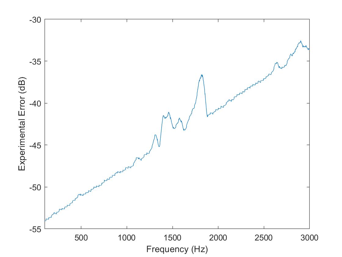
In order to filter out low-frequency ambient noise during the final demo, a high-pass filter was built on the end of the amplifier using the same op-amp chip. After choosing the capacitor and resistor values to have a filter cutoff frequency of about 600 Hz, we applied those values to the earlier LTSpice simulations and compared the Bode plot from the simulation to experimental data. We measured the output of the full microphone circuit and divided it by the input to the filter part of the circuit to find the transfer function of the filter and plot it on the same graph as the simulation Bode plot, shown below on the left. We then subtracted the simulated data from the experimental data to find the error, as shown below to the right.
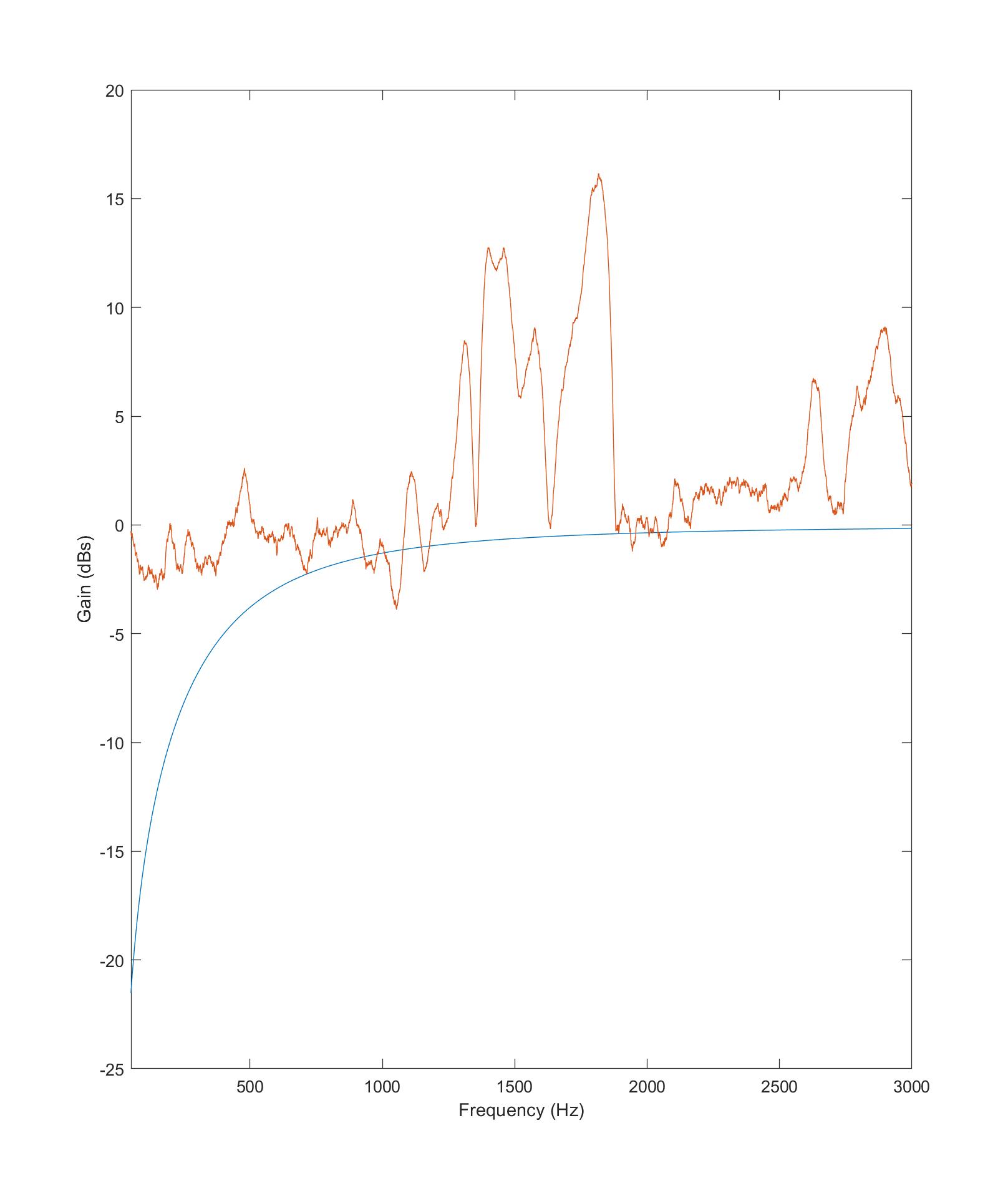
We encountered a couple issues with this part of the lab; at first, we were taking the input from before the amplifier as opposed to before the filter, so our transfer function was very different from our filter simulation due to the amplification. However, even after we measured the input from directly before the filter, there still appeared to be gain over the filter, as demonstrated by the positive decibel values shown on the experimental plot, compared to the 0 dB (no gain) values past the cuttoff frequency on the simulated plot.
Part 4: FFT on Arduino
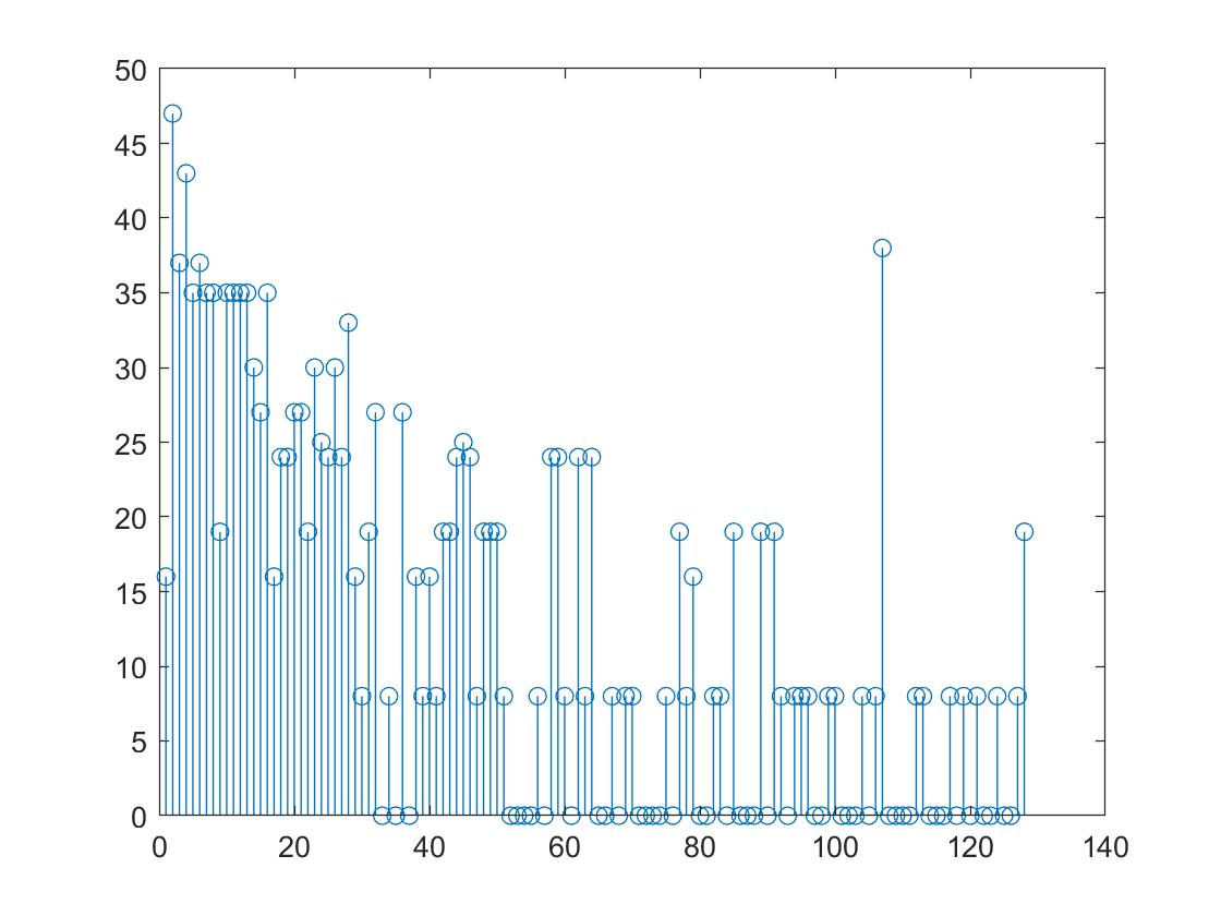
The final part of this lab was coding the FFT on the Arduino, as the robot will not be connected to a computer to use Matlab for the FFT in the final demo, but we need to have the capability to amplify, filter, and detect frequencies to start our tasks. To do this, we coded the Arduino to use interrupts to sample 256 values from the ADC, which was still running in free-running mode, at time intervals of 0.41667 ms. These values were then processed by the FFT library on the Arduino, and for testing purposes, these values were copied into Matlab and plotted against bins representing a small range of frequencies.
This part of the lab was by far the most problematic. When we first uploaded our interrupt service routine (ISR) code to the Arduino, the data we received and plotted in Matlab did not demonstrate the Arduino was detecting a peak at the frequency we played. An example of such a plot is shown below to the left. When we went back and re-ran previous code to ensure our circuit was still working, we found the FFT spectrum in Matlab to be extremely strange and also not indicative of correct frequency detection (shown below to the right). We even went back to reading the serial monitor's output in response to us tapping on the mic or playing certain tones, and the serial monitor often showed the mic was not detecting sound at all.
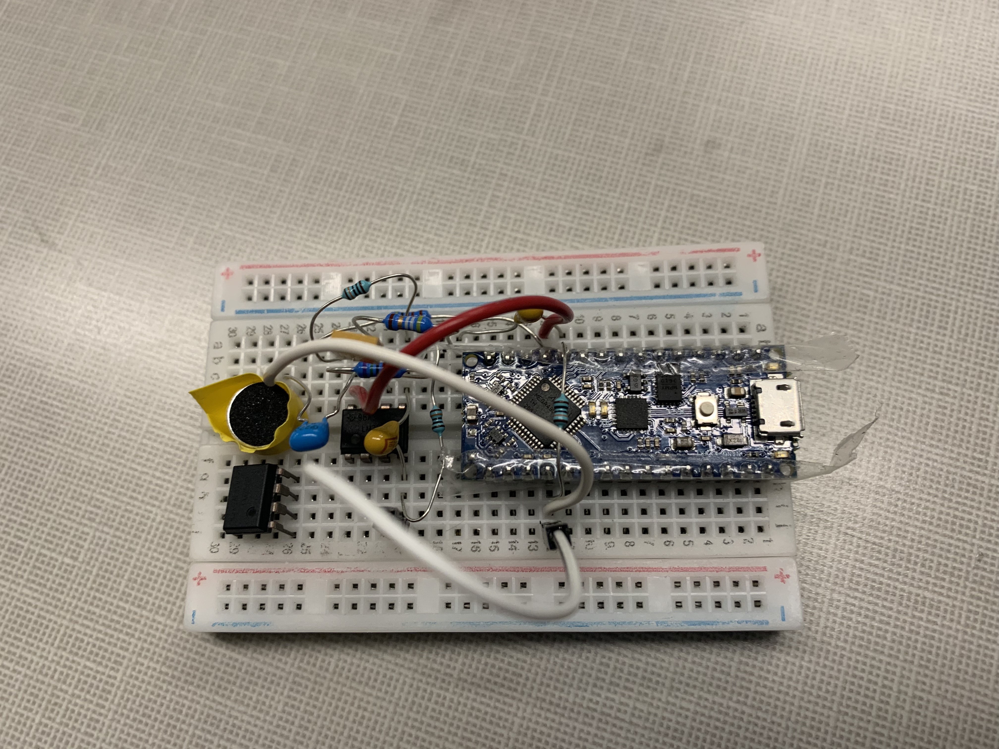
To try to find the source of this problem, we rebuilt the entire circuit on small breadboard using new Arduino and new components. After realizing the mic was not grounded, we had success with the basic mic circuit without amplification. We then built the amplification circuit and saw peaks smaller than what was on the non-amplified graph; after meticulously checking the circuit, we found that the resistor touching the mic's conductive package caused problems, and we saw a high peak once the signal was correctly amplified. However, as soon as we uploaded our ISR code again (without changing the circuit at all), we saw the same issues as before.
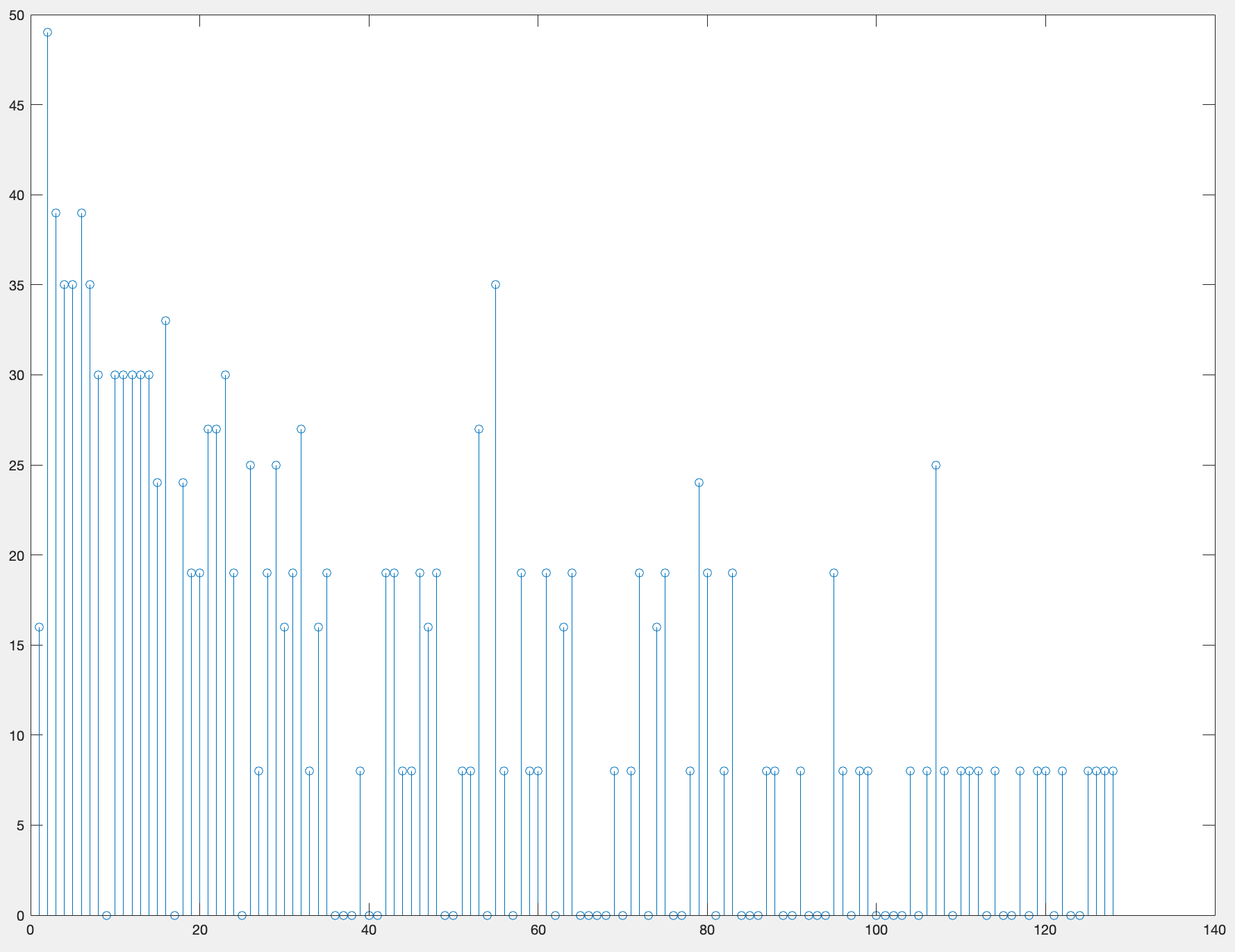
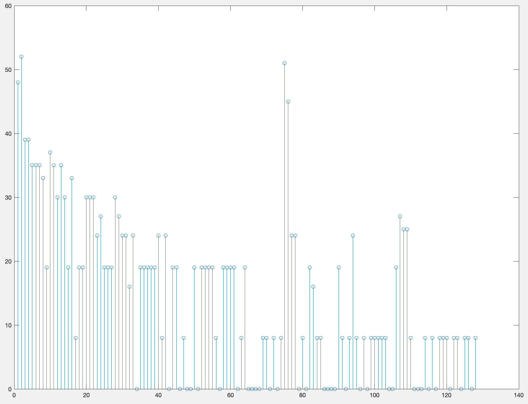
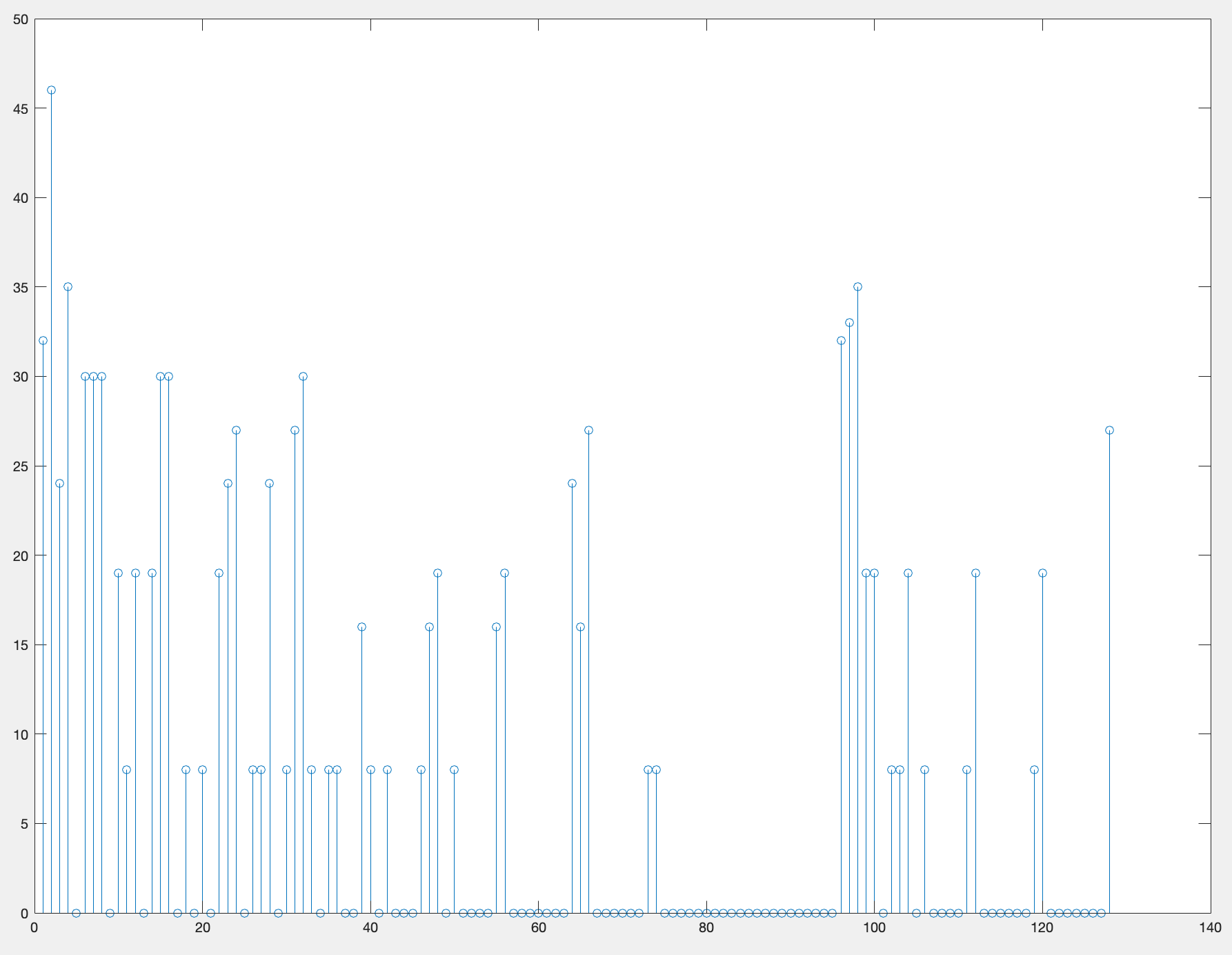
We eventually replaced the Arduino once more, and after using example code and after conducting a lot of testing, the FFT on the Arduino seemingly-coincidentally worked. This leads us to believe there were multiple factors contributing to the problem, including with our own code and how we modified the example code to work with our circuit. Plots corresponding to a frequency of 500 Hz (about bin 50), 700 Hz (near bin 80), and 900 Hz (near bin 100) are shown below.