library(tidyverse)
library(skimr)Data Analysis of Severe Crimes Committed in New York City
Appendix to report
Data cleaning
Rows: 189774 Columns: 19
── Column specification ────────────────────────────────────────────────────────
Delimiter: ","
chr (10): ARREST_DATE, PD_DESC, OFNS_DESC, LAW_CODE, LAW_CAT_CD, ARREST_BORO...
dbl  (9): ARREST_KEY, PD_CD, KY_CD, ARREST_PRECINCT, JURISDICTION_CODE, X_CO...

ℹ Use `spec()` to retrieve the full column specification for this data.
ℹ Specify the column types or set `show_col_types = FALSE` to quiet this message.
Warning: Using an external vector in selections was deprecated in tidyselect 1.1.0.
ℹ Please use `all_of()` or `any_of()` instead.
# Was:
data %>% select(drop_cols)
# Now:
data %>% select(all_of(drop_cols))
See <https://tidyselect.r-lib.org/reference/faq-external-vector.html>.# A tibble: 186,784 × 17
arrest_month arrest_day arrest_year offense_description level_of_offense
<int> <int> <int> <chr> <chr>
1 1 23 2022 JOSTLING M
2 1 31 2022 ROBBERY F
3 2 1 2022 FELONY ASSAULT F
4 2 13 2022 ASSAULT 3 & RELATED OFF… M
5 2 21 2022 ROBBERY F
6 3 14 2022 FELONY ASSAULT F
7 3 22 2022 FELONY ASSAULT F
8 3 29 2022 OFFENSES INVOLVING FRAUD M
9 4 5 2022 RAPE F
10 5 4 2022 FELONY ASSAULT F
# ℹ 186,774 more rows
# ℹ 12 more variables: arrest_boro <chr>, arrest_precinct <dbl>,
# jurisdiction_code <dbl>, age_group <fct>, gender <chr>, race <chr>,
# x_coord_cd <dbl>, y_coord_cd <dbl>, latitude <dbl>, longitude <dbl>,
# severe_crime <fct>, arrest_borough <chr># A tibble: 186,784 × 17
arrest_month arrest_day arrest_year offense_description level_of_offense
<int> <int> <int> <chr> <chr>
1 1 23 2022 JOSTLING M
2 1 31 2022 ROBBERY F
3 2 1 2022 FELONY ASSAULT F
4 2 13 2022 ASSAULT 3 & RELATED OFF… M
5 2 21 2022 ROBBERY F
6 3 14 2022 FELONY ASSAULT F
7 3 22 2022 FELONY ASSAULT F
8 3 29 2022 OFFENSES INVOLVING FRAUD M
9 4 5 2022 RAPE F
10 5 4 2022 FELONY ASSAULT F
# ℹ 186,774 more rows
# ℹ 12 more variables: arrest_boro <chr>, arrest_precinct <dbl>,
# jurisdiction_code <dbl>, age_group <fct>, gender <chr>, race <chr>,
# x_coord_cd <dbl>, y_coord_cd <dbl>, latitude <dbl>, longitude <dbl>,
# severe_crime <fct>, arrest_borough <chr>EDA
arrest_clean |>
  summarize(
    avg_arrest_month = mean(arrest_month),
    sd_arrest_month = sd(arrest_month),
    med_arrest_month = median(arrest_month)
  )
# A tibble: 1 × 3
avg_arrest_month sd_arrest_month med_arrest_month
<dbl> <dbl> <dbl>
1 6.62 3.39 7arrest_clean |>
ggplot(
mapping = aes(x = arrest_month)
) +
geom_bar()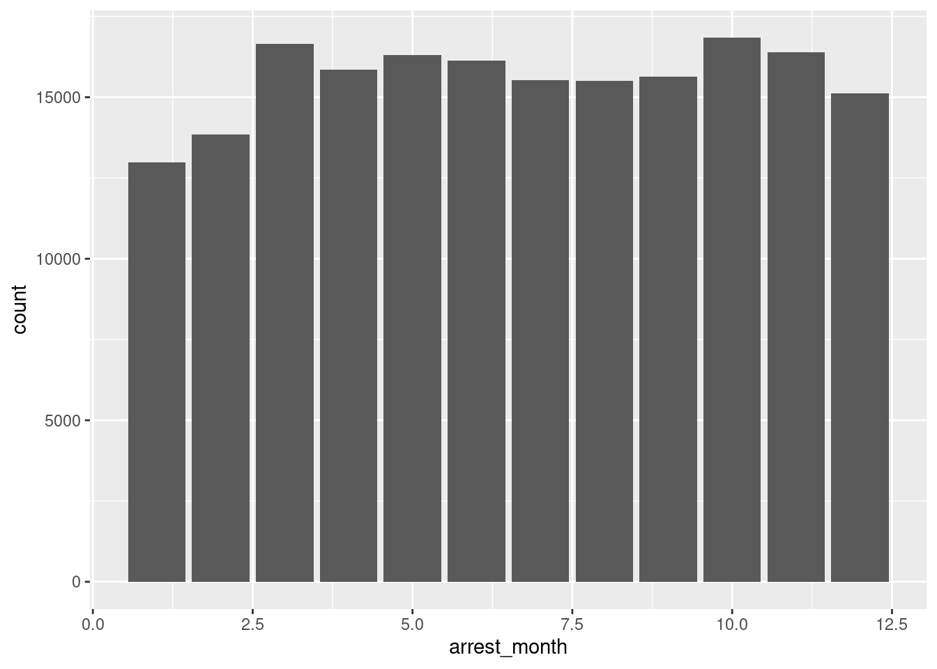
arrest_clean |>
  summarize(
    avg_arrest_day = mean(arrest_day),
    sd_arrest_day = sd(arrest_day),
    med_arrest_day = median(arrest_day)
  )
# A tibble: 1 × 3
avg_arrest_day sd_arrest_day med_arrest_day
<dbl> <dbl> <dbl>
1 15.5 8.75 15arrest_clean |>
ggplot(
mapping = aes(x = arrest_day)
) +
geom_bar()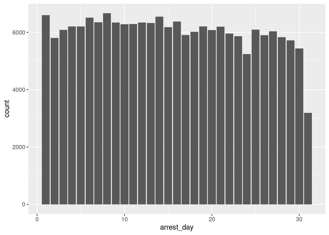
offense_descr_count <- arrest_clean |>
  group_by(offense_description) |>
  count(offense_description)
offense_descr_count
# A tibble: 64 × 2
# Groups: offense_description [64]
offense_description n
<chr> <int>
1 ADMINISTRATIVE CODE 126
2 ADMINISTRATIVE CODES 1
3 AGRICULTURE & MRKTS LAW-UNCLASSIFIED 73
4 ALCOHOLIC BEVERAGE CONTROL LAW 146
5 ANTICIPATORY OFFENSES 20
6 ARSON 144
7 ASSAULT 3 & RELATED OFFENSES 30582
8 BURGLAR'S TOOLS 568
9 BURGLARY 6231
10 CANNABIS RELATED OFFENSES 125
# ℹ 54 more rowsoffense_descr_level_count <- arrest_clean |>
group_by(offense_description, level_of_offense) |>
count(offense_description)
offense_descr_level_count# A tibble: 86 × 3
# Groups: offense_description, level_of_offense [86]
offense_description level_of_offense n
<chr> <chr> <int>
1 ADMINISTRATIVE CODE I 7
2 ADMINISTRATIVE CODE M 34
3 ADMINISTRATIVE CODE V 85
4 ADMINISTRATIVE CODES V 1
5 AGRICULTURE & MRKTS LAW-UNCLASSIFIED M 73
6 ALCOHOLIC BEVERAGE CONTROL LAW M 146
7 ANTICIPATORY OFFENSES M 20
8 ARSON F 144
9 ASSAULT 3 & RELATED OFFENSES M 30582
10 BURGLAR'S TOOLS M 568
# ℹ 76 more rowsarrest_clean |>
summarize(
avg_longitude = mean(longitude),
med_longitude = median(longitude),
sd_longitude = sd(longitude),
avg_latitude = mean(latitude),
med_latitude = median(latitude),
sd_latitude = sd(latitude),
)# A tibble: 1 × 6
avg_longitude med_longitude sd_longitude avg_latitude med_latitude sd_latitude
<dbl> <dbl> <dbl> <dbl> <dbl> <dbl>
1 -73.9 -73.9 0.0762 40.7 40.7 0.0814arrest_clean |>
ggplot(aes(x = longitude, y = latitude)) +
geom_point(size = .25, show.legend = FALSE) +
coord_quickmap()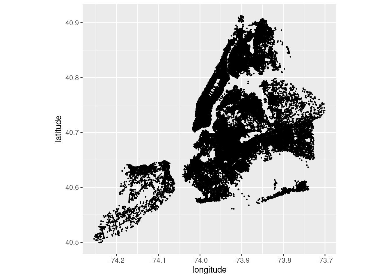
arrest_clean |>
  group_by(offense_description, level_of_offense, age_group) |>
  count(offense_description)
# A tibble: 344 × 4
# Groups: offense_description, level_of_offense, age_group [344]
offense_description level_of_offense age_group n
<chr> <chr> <fct> <int>
1 ADMINISTRATIVE CODE I 18-24 1
2 ADMINISTRATIVE CODE I 25-44 3
3 ADMINISTRATIVE CODE I 45-64 2
4 ADMINISTRATIVE CODE I 65+ 1
5 ADMINISTRATIVE CODE M 18-24 1
6 ADMINISTRATIVE CODE M 25-44 18
7 ADMINISTRATIVE CODE M 45-64 13
8 ADMINISTRATIVE CODE M 65+ 2
9 ADMINISTRATIVE CODE V 18-24 10
10 ADMINISTRATIVE CODE V 25-44 50
# ℹ 334 more rows#Number of offenses committed by each age group
age_counts <- arrest_clean |>
group_by(age_group) |>
summarise(num_offenses = n())
age_counts# A tibble: 5 × 2
age_group num_offenses
<fct> <int>
1 <18 6770
2 18-24 32705
3 25-44 107415
4 45-64 37056
5 65+ 2838# Bar graph of age group vs. number of offenses
ggplot(age_counts, aes(x = age_group, y = num_offenses)) +
geom_bar(stat = "identity") +
labs(
x = "Age group",
y = "Number of offenses",
title = "Number of offenses by Age Group"
) 
#Number of offenses committed by each age group-race
age_counts <- arrest_clean |>
  group_by(age_group, race) |>
  summarise(num_offenses = n())
`summarise()` has grouped output by 'age_group'. You can override using the
`.groups` argument.age_counts# A tibble: 30 × 3
# Groups: age_group [5]
age_group race num_offenses
<fct> <chr> <int>
1 <18 AMERICAN INDIAN/ALASKAN NATIVE 15
2 <18 ASIAN / PACIFIC ISLANDER 266
3 <18 BLACK 4091
4 <18 BLACK HISPANIC 735
5 <18 WHITE 305
6 <18 WHITE HISPANIC 1358
7 18-24 AMERICAN INDIAN/ALASKAN NATIVE 102
8 18-24 ASIAN / PACIFIC ISLANDER 1560
9 18-24 BLACK 16992
10 18-24 BLACK HISPANIC 3592
# ℹ 20 more rows# Bar graph of age group vs. number of offenses by race
ggplot(age_counts, aes(x = age_group, y = num_offenses)) +
geom_bar(stat = "identity") +
labs(
x = "Age group",
y = "Number of offenses",
title = "Number of offenses by age group and race"
) +
facet_wrap(vars(race))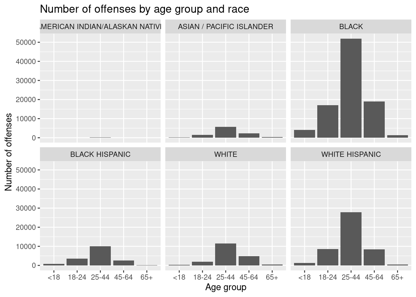
race_count <- arrest_clean |>
  group_by(race) |>
  count(race) |>
  mutate(percentage = 100*n/189774)
race_count
# A tibble: 6 × 3
# Groups: race [6]
race n percentage
<chr> <int> <dbl>
1 AMERICAN INDIAN/ALASKAN NATIVE 516 0.272
2 ASIAN / PACIFIC ISLANDER 10085 5.31
3 BLACK 93229 49.1
4 BLACK HISPANIC 17139 9.03
5 WHITE 19158 10.1
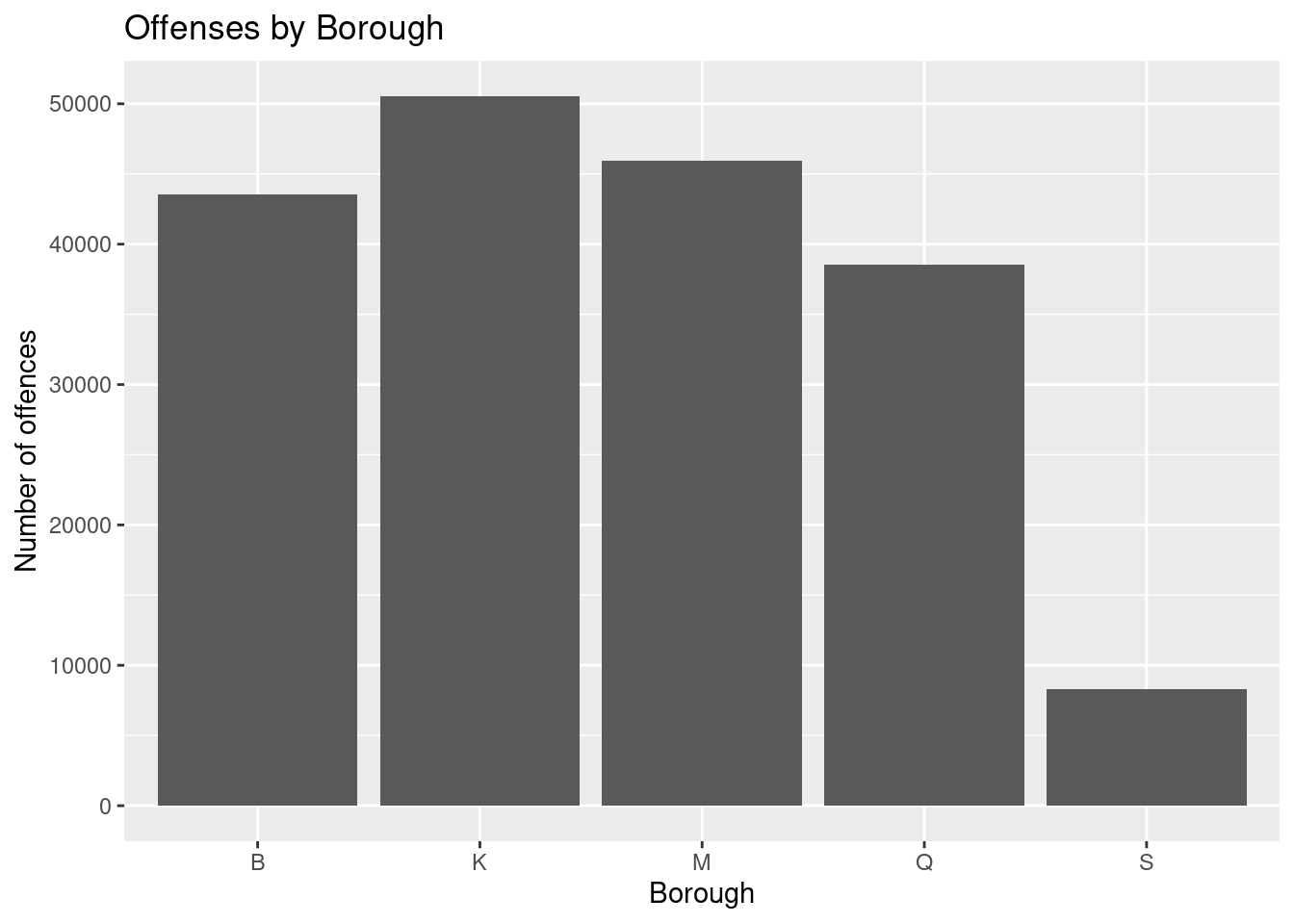
6 WHITE HISPANIC 46657 24.6 borough_counts <- arrest_clean |>
group_by(arrest_boro) |>
count()
borough_counts# A tibble: 5 × 2
# Groups: arrest_boro [5]
arrest_boro n
<chr> <int>
1 B 43519
2 K 50531
3 M 45945
4 Q 38511
5 S 8278# plot a bar graph of borough vs. number of offenses
ggplot(borough_counts, aes(x = arrest_boro, y = n)) +
geom_bar(stat = "identity") +
labs(
x = "Borough",
y = "Number of offences",
title = "Offenses by Borough"
) 
Spatial Data Analysis
latitudes = seq(40.49939, 40.91296, by = 0.41357/28.530)
longitudes = seq(-74.25422, -73.70072, by = 0.5535/28.530)
arrest_grouped <- arrest_clean |>
  mutate(
    grid_cell = cut(
      arrest_clean$latitude,
      breaks = latitudes, labels = FALSE
    ) +
      (cut(
        arrest_clean$longitude,
        breaks = longitudes,
        labels = FALSE) - 1) * length(latitudes),
    grid_cell = factor(grid_cell)
  ) |>
  group_by(grid_cell) |>
  filter(severe_crime == "Yes")|>
  summarize(
    avg_lat = mean(latitude),
    avg_long = mean(longitude),
    min_lat = min(latitude),
    max_lat = max(latitude),
    min_long = min(longitude),
    max_long = max(longitude),
    num_severe_crimes = n(),
    common_boro = names(sort(-table(arrest_borough)))[1]
  )

arrest_grouped |>
  head(5)
# A tibble: 5 × 9
grid_cell avg_lat avg_long min_lat max_lat min_long max_long num_severe_crimes
<fct> <dbl> <dbl> <dbl> <dbl> <dbl> <dbl> <int>
1 1 40.5 -74.2 40.5 40.5 -74.3 -74.2 119
2 2 40.5 -74.2 40.5 40.5 -74.2 -74.2 13
3 3 40.5 -74.2 40.5 40.5 -74.2 -74.2 3
4 30 40.5 -74.2 40.5 40.5 -74.2 -74.2 6
5 31 40.5 -74.2 40.5 40.5 -74.2 -74.2 12
# ℹ 1 more variable: common_boro <chr>Summary Statistics by Grid
arrest_grouped |>
  ggplot(
    aes(
      x = avg_long,
      y = avg_lat,
      size = num_severe_crimes,
      color = common_boro)) +
  geom_point(alpha = 0.5) +
  scale_size(guide = "none") +
  coord_quickmap() +
  labs(
    x = "Longitude(°)",
    y = "Latitude(°)",
    title = "Severe Crimes in New York City",
    color = "Borough"
  ) +
  theme_minimal() +
  theme(
    plot.title = element_text(size = 20)
)