library(tidyverse)
library(skimr)Data Analysis of Severe Crimes Committed in New York City
Exploratory data analysis
Research question(s)
Research question(s). State your research question (s) clearly.
What demographic groups within different boroughs of New York City can be identified as “most dangerous”? Is there a day of the month or month of the year where these boroughs are most dangerous/have the most crime? What crimes are most committed in different boroughs?
Data collection and cleaning
Have an initial draft of your data cleaning appendix. Document every step that takes your raw data file(s) and turns it into the analysis-ready data set that you would submit with your final project. Include text narrative describing your data collection (downloading, scraping, surveys, etc) and any additional data curation/cleaning (merging data frames, filtering, transformations of variables, etc). Include code for data curation/cleaning, but not collection.
Rows: 189774 Columns: 19
── Column specification ────────────────────────────────────────────────────────
Delimiter: ","
chr (10): ARREST_DATE, PD_DESC, OFNS_DESC, LAW_CODE, LAW_CAT_CD, ARREST_BORO...
dbl  (9): ARREST_KEY, PD_CD, KY_CD, ARREST_PRECINCT, JURISDICTION_CODE, X_CO...

ℹ Use `spec()` to retrieve the full column specification for this data.
ℹ Specify the column types or set `show_col_types = FALSE` to quiet this message.
Warning: Using an external vector in selections was deprecated in tidyselect 1.1.0.
ℹ Please use `all_of()` or `any_of()` instead.
# Was:
data %>% select(drop_cols)
# Now:
data %>% select(all_of(drop_cols))
See <https://tidyselect.r-lib.org/reference/faq-external-vector.html>.# A tibble: 186,784 × 17
arrest_month arrest_day arrest_year offense_description level_of_offense
<int> <int> <int> <chr> <chr>
1 1 23 2022 JOSTLING M
2 1 31 2022 ROBBERY F
3 2 1 2022 FELONY ASSAULT F
4 2 13 2022 ASSAULT 3 & RELATED OFF… M
5 2 21 2022 ROBBERY F
6 3 14 2022 FELONY ASSAULT F
7 3 22 2022 FELONY ASSAULT F
8 3 29 2022 OFFENSES INVOLVING FRAUD M
9 4 5 2022 RAPE F
10 5 4 2022 FELONY ASSAULT F
# ℹ 186,774 more rows
# ℹ 12 more variables: arrest_boro <chr>, arrest_precinct <dbl>,
# jurisdiction_code <dbl>, age_group <fct>, gender <chr>, race <chr>,
# x_coord_cd <dbl>, y_coord_cd <dbl>, latitude <dbl>, longitude <dbl>,
# severe_crime <fct>, arrest_borough <chr>Data description
Have an initial draft of your data description section. Your data description should be about your analysis-ready data.
What are the observations (rows) and the attributes (columns)?
- Each row represents an arrest record that occurred in New York State from 2020. The columns represent the details of the arrest such as the demographics of the offender, the degree of crime, and details of the location it occurred.
Why was this dataset created?
- The dataset was created so that the public can explore the nature of police enforcement activity. Citizens who view this data be aware day by day in what regions what types of activities the NYPD has done regarding arresting offenders.
What processes might have influenced what data was observed and recorded and what was not?
The website from which the datset is from states that data is manually extracted every quarter and reviewed by the Office of Management. This shows that there is some process that is not revealed to the public regarding how the NYPD manages their raw data, and shows how the dataset we are using is already filtered first. There is a high chance that very minor arrests may have been filtered out as deemed insignificant by the Office of Management.
Some factors that may have influenced what data was observed are NY policing practices. The number of police that are out in New York State is probably not equal in every area as the number probably correlates highly with the population density and crime rates of the area. This may have resulted in more arrest records in areas that were already high in crime rates to be recorded.
External factors such as politics may also play a role in this dataset because if certain policies pressure the police department to reduce crime rates, the number of rows in the dataset may probably increase and vice versa.
What preprocessing was done, and how did the data come to be in the form that you are using?
- Initially, we went through each data variable that was part of the entire dataset and removed irrelevant and unnecessary variables that do not pertain to our research question. We generally kept potential variables that could be used regarding the type of offense, precinct number, severity, etc. Our data is in the form that we are using because we are trying to analyze the impact on age and location on most dangerous crimes. We compared the different variables with each other to find possible correlations so that we can further analyze and answer our research question.
If people are involved, were they aware of the data collection and if so, what purpose did they expect the data to be used for?
- Specific people weren’t named in the data collection, however, only official police reports within NYC was part of this data. They probably did not report for their data to be collected for analyzing, but generally the police will use the data to see how to combat certain crimes in certain regions.
Data limitations
Identify any potential problems with your dataset.
One of the limitations in the dataset is that the sample is not representative of the true demographics of New York City. According to 2022 data, the race breakdown of NYC is approximately 40% White, 23.4% Black, 14.2% Asian, and 28.9% Hispanic. However, the demographic samples in our data don’t have similar percentages, with the amount of Black people surveyed being disproportionately large at 49.6%. This may cause some bias in the results of our data analysis. Another limitation in the dataset could be that not all the crimes may be part of the dataset in that many cases can happen and not be reported. In 2006 to 2010, 3 in 10 crimes involving injury and a weapon went unreported and not noted to the police in NYC, which can hinder the data set from being fully accurate.
Exploratory data analysis
Perform an (initial) exploratory data analysis.
arrest_clean |>
  summarize(
    avg_arrest_month = mean(arrest_month),
    sd_arrest_month = sd(arrest_month),
    med_arrest_month = median(arrest_month)
  )
# A tibble: 1 × 3
avg_arrest_month sd_arrest_month med_arrest_month
<dbl> <dbl> <dbl>
1 6.62 3.39 7arrest_clean |>
ggplot(
mapping = aes(x = arrest_month)
) +
geom_bar()
arrest_clean |>
  summarize(
    avg_arrest_day = mean(arrest_day),
    sd_arrest_day = sd(arrest_day),
    med_arrest_day = median(arrest_day)
  )
# A tibble: 1 × 3
avg_arrest_day sd_arrest_day med_arrest_day
<dbl> <dbl> <dbl>
1 15.5 8.75 15arrest_clean |>
ggplot(
mapping = aes(x = arrest_day)
) +
geom_bar()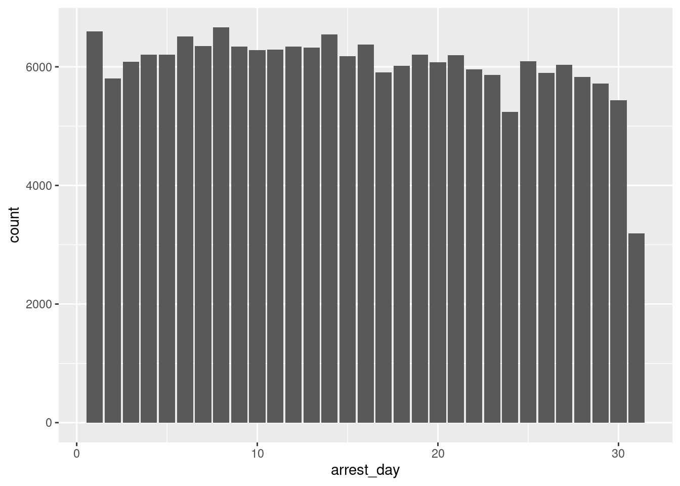
offense_descr_count <- arrest_clean |>
  group_by(offense_description) |>
  count(offense_description)
offense_descr_count
# A tibble: 64 × 2
# Groups: offense_description [64]
offense_description n
<chr> <int>
1 ADMINISTRATIVE CODE 126
2 ADMINISTRATIVE CODES 1
3 AGRICULTURE & MRKTS LAW-UNCLASSIFIED 73
4 ALCOHOLIC BEVERAGE CONTROL LAW 146
5 ANTICIPATORY OFFENSES 20
6 ARSON 144
7 ASSAULT 3 & RELATED OFFENSES 30582
8 BURGLAR'S TOOLS 568
9 BURGLARY 6231
10 CANNABIS RELATED OFFENSES 125
# ℹ 54 more rowsoffense_descr_level_count <- arrest_clean |>
group_by(offense_description, level_of_offense) |>
count(offense_description)
offense_descr_level_count# A tibble: 86 × 3
# Groups: offense_description, level_of_offense [86]
offense_description level_of_offense n
<chr> <chr> <int>
1 ADMINISTRATIVE CODE I 7
2 ADMINISTRATIVE CODE M 34
3 ADMINISTRATIVE CODE V 85
4 ADMINISTRATIVE CODES V 1
5 AGRICULTURE & MRKTS LAW-UNCLASSIFIED M 73
6 ALCOHOLIC BEVERAGE CONTROL LAW M 146
7 ANTICIPATORY OFFENSES M 20
8 ARSON F 144
9 ASSAULT 3 & RELATED OFFENSES M 30582
10 BURGLAR'S TOOLS M 568
# ℹ 76 more rowsarrest_clean |>
summarize(
avg_longitude = mean(longitude),
med_longitude = median(longitude),
sd_longitude = sd(longitude),
avg_latitude = mean(latitude),
med_latitude = median(latitude),
sd_latitude = sd(latitude),
)# A tibble: 1 × 6
avg_longitude med_longitude sd_longitude avg_latitude med_latitude sd_latitude
<dbl> <dbl> <dbl> <dbl> <dbl> <dbl>
1 -73.9 -73.9 0.0762 40.7 40.7 0.0814arrest_clean |>
ggplot(aes(x = longitude, y = latitude)) +
geom_point(size = .25, show.legend = FALSE) +
coord_quickmap()
# does not work
# newyork_map <- get_stamenmap(
#  bbox = c(left = -77.036, bottom = 41.459, right = -69.478, top = 44.040),
#  maptype = "terrain",
#  zoom = 7
#)
arrest_clean |>
group_by(offense_description, level_of_offense, age_group) |>
count(offense_description)# A tibble: 344 × 4
# Groups: offense_description, level_of_offense, age_group [344]
offense_description level_of_offense age_group n
<chr> <chr> <fct> <int>
1 ADMINISTRATIVE CODE I 18-24 1
2 ADMINISTRATIVE CODE I 25-44 3
3 ADMINISTRATIVE CODE I 45-64 2
4 ADMINISTRATIVE CODE I 65+ 1
5 ADMINISTRATIVE CODE M 18-24 1
6 ADMINISTRATIVE CODE M 25-44 18
7 ADMINISTRATIVE CODE M 45-64 13
8 ADMINISTRATIVE CODE M 65+ 2
9 ADMINISTRATIVE CODE V 18-24 10
10 ADMINISTRATIVE CODE V 25-44 50
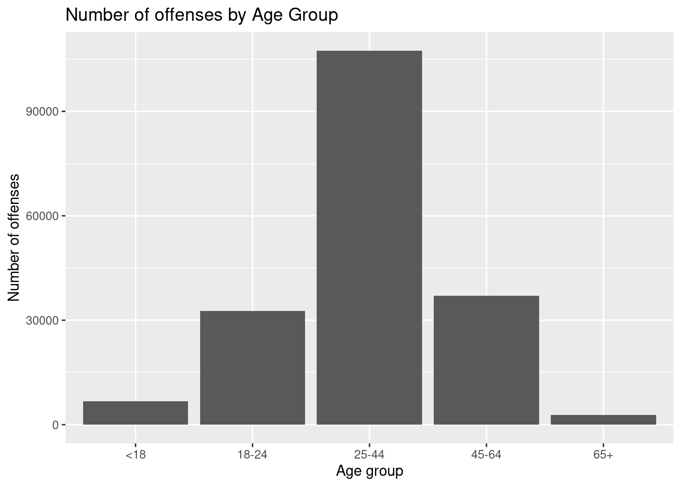
# ℹ 334 more rows#Number of offenses committed by each age group
age_counts <- arrest_clean |>
group_by(age_group) |>
summarise(num_offenses = n())
age_counts# A tibble: 5 × 2
age_group num_offenses
<fct> <int>
1 <18 6770
2 18-24 32705
3 25-44 107415
4 45-64 37056
5 65+ 2838# Bar graph of age group vs. number of offenses
ggplot(age_counts, aes(x = age_group, y = num_offenses)) +
geom_bar(stat = "identity") +
labs(
x = "Age group",
y = "Number of offenses",
title = "Number of offenses by Age Group"
) 
#Number of offenses committed by each age group-race
age_counts <- arrest_clean |>
  group_by(age_group, race) |>
  summarise(num_offenses = n())
`summarise()` has grouped output by 'age_group'. You can override using the
`.groups` argument.age_counts# A tibble: 30 × 3
# Groups: age_group [5]
age_group race num_offenses
<fct> <chr> <int>
1 <18 AMERICAN INDIAN/ALASKAN NATIVE 15
2 <18 ASIAN / PACIFIC ISLANDER 266
3 <18 BLACK 4091
4 <18 BLACK HISPANIC 735
5 <18 WHITE 305
6 <18 WHITE HISPANIC 1358
7 18-24 AMERICAN INDIAN/ALASKAN NATIVE 102
8 18-24 ASIAN / PACIFIC ISLANDER 1560
9 18-24 BLACK 16992
10 18-24 BLACK HISPANIC 3592
# ℹ 20 more rows# Bar graph of age group vs. number of offenses by race
ggplot(age_counts, aes(x = age_group, y = num_offenses)) +
geom_bar(stat = "identity") +
labs(
x = "Age group",
y = "Number of offenses",
title = "Number of offenses by age group and race"
) +
facet_wrap(vars(race))
race_count <- arrest_clean |>
  group_by(race) |>
  count(race) |>
  mutate(percentage = 100*n/189774)
race_count
# A tibble: 6 × 3
# Groups: race [6]
race n percentage
<chr> <int> <dbl>
1 AMERICAN INDIAN/ALASKAN NATIVE 516 0.272
2 ASIAN / PACIFIC ISLANDER 10085 5.31
3 BLACK 93229 49.1
4 BLACK HISPANIC 17139 9.03
5 WHITE 19158 10.1
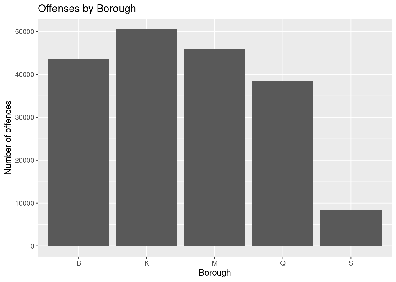
6 WHITE HISPANIC 46657 24.6 borough_counts <- arrest_clean |>
group_by(arrest_boro) |>
count()
borough_counts# A tibble: 5 × 2
# Groups: arrest_boro [5]
arrest_boro n
<chr> <int>
1 B 43519
2 K 50531
3 M 45945
4 Q 38511
5 S 8278# plot a bar graph of borough vs. number of offenses
ggplot(borough_counts, aes(x = arrest_boro, y = n)) +
geom_bar(stat = "identity") +
labs(
x = "Borough",
y = "Number of offences",
title = "Offenses by Borough"
) 
Questions for reviewers
List specific questions for your peer reviewers and project mentor to answer in giving you feedback on this phase.
Does time (month or day of the month) have a correlation to criminal activity?
Is there a specific age group that tends to participate in criminal activity more frequently?
Is our updated research question specific yet broad enough for the scope of this project?
How many variables should we incorporate to be sufficient for this project?
Is there a specific format that the data description should be altered for the later portion of the project?