# Load library(s) and data
library(tidyverse)
library(skimr)
library(viridis)
library(scales)
bills <- read_csv("data/billionaires.csv")Characteristics of Billionaires
Exploratory data analysis
Research question(s)
Research question(s). State your research question (s) clearly.
- How do the demographics age and gender play a role in the number of billionaires across the different regions in 2014?
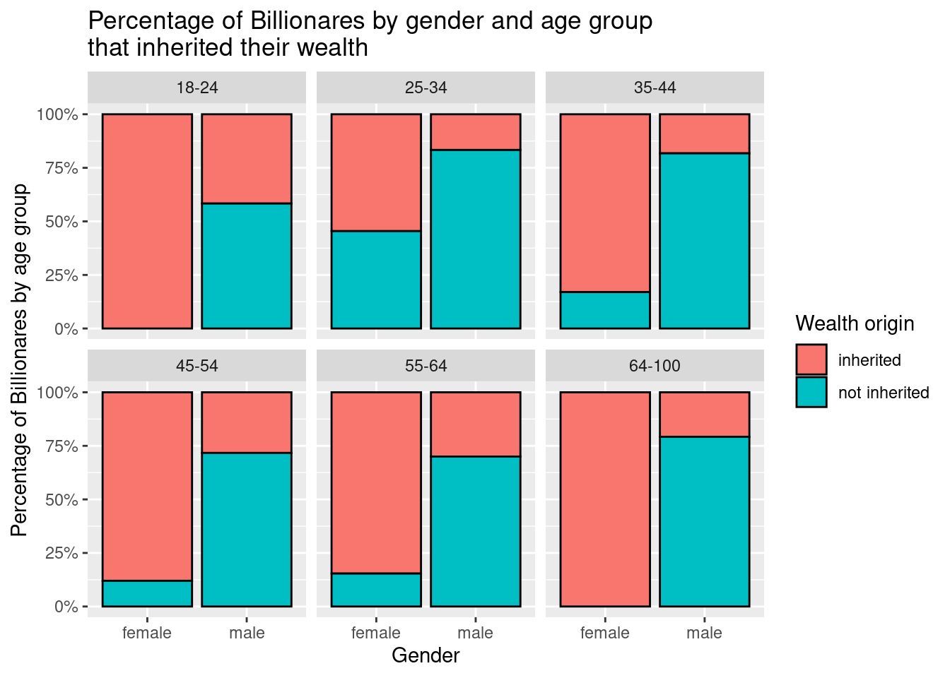
- Do age and gender also play a role in the inheritance of wealth among billionaires based on the data from 2014?
Data collection and cleaning
Have an initial draft of your data cleaning appendix. Document every step that takes your raw data file(s) and turns it into the analysis-ready data set that you would submit with your final project. Include text narrative describing your data collection (downloading, scraping, surveys, etc) and any additional data curation/cleaning (merging data frames, filtering, transformations of variables, etc). Include code for data curation/cleaning, but not collection.
bills_clean <- bills |>
  # filtering to get only 2014 data
  filter(year == 2014) |>
  # selecting relevant variables
  select(name, demographics.age, demographics.gender,
         location.region, wealth.how.inherited) |>
  # renaming columns to meet style guidelines
  rename(
    age = demographics.age,
    gender = demographics.gender,
    region = location.region,
    inheritance = wealth.how.inherited
  ) |>
  # filtering out billionares with 0 age
  filter(!age == 0) |>
  # adding age range column
  mutate(
    age_range = cut_interval(age, n=6,
                  labels = c("18-24", "25-34",
                             "35-44", "45-54",
                             "55-64", "64-100")

  )
  )


# separating inherited variable into "inherited" and "not inherited"
bills_clean$inheritance <- ifelse(
  bills_clean$inheritance %in% "not inherited", "not inherited", "inherited"
)


bills_clean
# A tibble: 1,590 × 6
name age gender region inheritance age_range
<chr> <dbl> <chr> <chr> <chr> <fct>
1 Bill Gates 58 male North America not inherited 35-44
2 Carlos Slim Helu 74 male Latin America not inherited 55-64
3 Amancio Ortega 77 male Europe not inherited 55-64
4 Warren Buffett 83 male North America not inherited 55-64
5 Larry Ellison 69 male North America not inherited 45-54
6 Charles Koch 78 male North America inherited 55-64
7 David Koch 73 male North America inherited 45-54
8 Sheldon Adelson 80 male North America not inherited 55-64
9 Christy Walton 59 female North America inherited 35-44
10 Jim Walton 66 male North America inherited 45-54
# ℹ 1,580 more rowsskim(bills_clean)| Name | bills_clean |
| Number of rows | 1590 |
| Number of columns | 6 |
| _______________________ | |
| Column type frequency: | |
| character | 4 |
| factor | 1 |
| numeric | 1 |
| ________________________ | |
| Group variables | None |
Variable type: character
| skim_variable | n_missing | complete_rate | min | max | empty | n_unique | whitespace |
|---|---|---|---|---|---|---|---|
| name | 0 | 1 | 5 | 45 | 0 | 1590 | 0 |
| gender | 0 | 1 | 4 | 6 | 0 | 2 | 0 |
| region | 0 | 1 | 6 | 24 | 0 | 7 | 0 |
| inheritance | 0 | 1 | 9 | 13 | 0 | 2 | 0 |
Variable type: factor
| skim_variable | n_missing | complete_rate | ordered | n_unique | top_counts |
|---|---|---|---|---|---|
| age_range | 0 | 1 | FALSE | 6 | 35-: 519, 45-: 495, 55-: 276, 25-: 196 |
Variable type: numeric
| skim_variable | n_missing | complete_rate | mean | sd | p0 | p25 | p50 | p75 | p100 | hist |
|---|---|---|---|---|---|---|---|---|---|---|
| age | 0 | 1 | 63.34 | 13.14 | 24 | 53 | 63 | 73 | 98 | ▁▅▇▆▂ |
Initial Draft of Data Cleaning Appendix:
We collected our data by downloading the csv file from the CORGIS Dataset Project online. We then uploaded the raw csv data and loaded it using read_csv(). From there, we began cleaning/curating our data to our research question. First, we filtered so that only data collected in 2014 remained, since our research question pertains to data collected in 2014 only. The original data set had data from 1996, 2001, and 2014, so some people, such as Bill Gates, were included multiple times. Filtering for only 2014 data prevents these people from being counted multiple times in our analysis. Next, we selected only the columns that are directly related to our research questions, which are age, gender, region, and inheritance, and kept name as an identifier variable, so that only relevant data is included in our data set and it is not overwhelmed by unused variables. Then, we renamed them to meet style guidelines and also to make them easier to use and understand. At this point, we realized that there were no NA values remaining in our data, but the age for some people was 0, which is clearly in lieu of it being NA. So, we filtered our data to get rid of these because they would skew the age analysis down inaccurately and they are not meaningful. Additionally, we added a variable age range based on the typical age ranges used in other analyses we have seen. We thought this variable would be useful, since there are so many different ages in our data that it would not be practical to do any analysis grouping by individual ages. Finally, we grouped the inheritance variable into two categories, “inherited” and “not inherited”. Now, our data has no NA values, has clean names and values, and is ready for analysis.
Data description
Have an initial draft of your data description section. Your data description should be about your analysis-ready data.
What are the observations (rows) and the attributes (columns)?
The attributes (columns) are billionaires’ name, age, gender, region, age_range, and inheritance. There are 7 regions, 6 age_range values, and 2 inheritance values. Each of the observations (rows) represents a billionaire in the dataset. (after data cleaning)
Why was this dataset created?
The dataset was created for a working paper from 2016 by Caroline Freund and Sarah Oliver for PIIE (Peterson Institute for International Economics). Researchers compiled a multi-decade database of the super-rich building off the Forbes World’s Billionaires lists from 1996-2014. The data serves to describe the factors related to why or how someone is a billionaire.
Who funded the creation of the dataset?
The Peterson Institute for International Economics funded the creation of the dataset.
What processes might have influenced what data was observed and recorded and what was not?
The data was observed and recorded based on Forbes World’s Billionaires list. Forbes may have overestimated or underestimated the wealth of individuals depending on their methodology for determining net worth, so this may have influenced which data was observed and recorded and who was disincluded. We also filtered the dataset to only keep the data from 2014, since a lot of observations have changed over time and we want to focus on a specific year to get an accurate result. We also selected the name, age, gender, region as the research variables we want to focus on, so this influenced what is included in our analysis-ready data.
What preprocessing was done, and how did the data come to be in the form that you are using?
We first filtered the original dataset to get only 2014 data. Then we selected the variables, name, demographics.age, demographics.gender, location.region, wealth.how.inherited, the variables we want to focus on, and renamed those columns to meet the style guideline. Finally we filtered out observations with age = 0, created a new age_range column that fit every observation into 6 age ranges, and separated the inheritance variable into 2 categories.
If people are involved, were they aware of the data collection and if so, what purpose did they expect the data to be used for?
There are people involved, as the whole dataset has to do with the billionaires of the world. There were no comments about whether these billionaires are aware of the data collection process. However, it is likely that most of it is public information available online.
Data limitations
Identify any potential problems with your dataset.
The original data set includes data collected from only 3 years: 1996, 2001, and 2014. Therefore, we thought that we could not properly investigate change over time or make predictions for the future with only 3 time points of data. However, we did originally want to do this and thought that perhaps the amount of time we are inlcuding is not enough. Since we are only analyzing 2014, this does not reflect change over time and may not produce super meaningful answers.
There may be billionaires that existed in 2014 but are not included in our data set, since some may keep their wealth private or may hold it illegally.
While our analysis of billionaires will hopefully reveal some trends in exterme wealth across the world, $1 billion is kind of an arbitrary threshold so our analysis may not fully characterize trends in extreme wealth other than billionaires.
Exploratory data analysis
Perform an (initial) exploratory data analysis.
# reorder plot by countries with the least 64-100 age range proportion in ascending order
bills_clean |>
  mutate(
    region = as.factor(region),
    region = fct_relevel(.f = region, "Sub-Saharan Africa", "South Asia", "Middle East/North Africa", "Europe", "East Asia", "Latin America", "North America")
  ) |>

# age_range visualization
ggplot(mapping = aes(x = region, fill = age_range)) +
  geom_bar(position = "fill", size = 0.5) +
  labs(x = "Region Location", y = "Age Range ", fill = "Age Range", title = "Relationship Between a Billionare's age range and \nWhat Region They Are From")+
  scale_x_discrete(guide=guide_axis(n.dodge=2))+
  theme_minimal() +
  theme(
    legend.position = "bottom",
    legend.direction = "horizontal"
  )
Warning: Using `size` aesthetic for lines was deprecated in ggplot2 3.4.0.
ℹ Please use `linewidth` instead.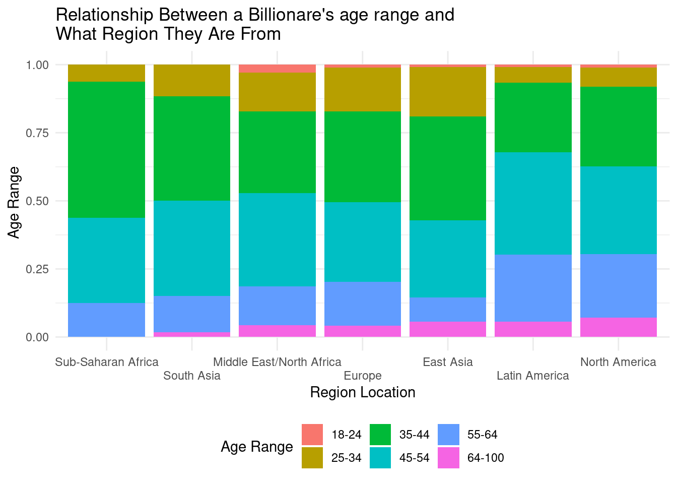
# reorder plot by countries with largest male proportion in desc order
bills_clean |>
  mutate(
    region = as.factor(region),
    region = fct_relevel(.f = region, "South Asia","East Asia","Middle East/North Africa","Europe","North America", "Sub-Saharan Africa", "Latin America")
  ) |>

# gender visualization
ggplot(mapping = aes(x = region, fill = gender)) +
  geom_bar(position = "fill", color = "black", size = 0.5) +
  labs(
      x = "Region Location",
      y = "Percentage of Billionares in Region",
      fill = "Gender of Billionare",
      title = "Relationship Between a Billionare's Gender and \nWhat Region They Are From"
    ) +
  scale_y_continuous(labels = label_percent()) +
  theme_minimal() +
  theme(
    legend.position = "bottom",
    legend.direction = "horizontal"
  ) +
  scale_x_discrete(guide=guide_axis(n.dodge=2)) +
  scale_fill_manual(labels = c("Female", "Male"),
                     values = c("pink", "lightblue"))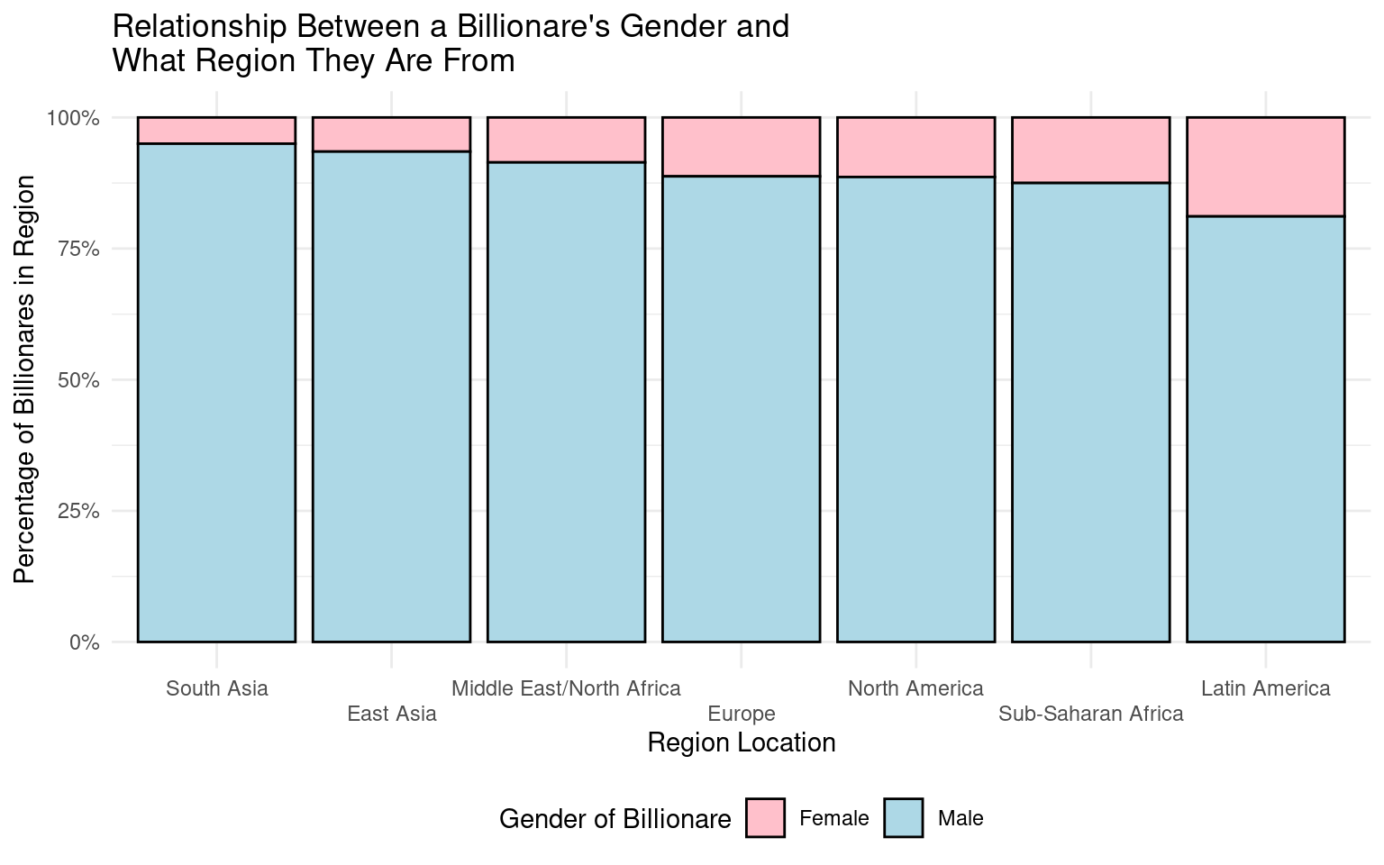
bills_clean |>
  mutate(age_range = fct_relevel(
    .f = age_range, "18-24", "25-34", "35-44", "45-54", "55-64", "64-100"
    )
  ) |>
  ggplot(aes(x= gender, fill= inheritance)) +
  geom_bar(position = "fill", color = "black", size = 0.5) +
  scale_y_continuous(labels = label_percent()) +
  facet_wrap(~ age_range)+
  labs(
    x= "Gender",
    y= "Percentage of Billionares by age group",
    title= "Percentage of Billionares by gender and age group \nthat inherited their wealth",
    fill= "Wealth origin"
  )
# counts based on one variable at a time
bills_clean |>
  count(region)
# A tibble: 7 × 2
region n
<chr> <int>
1 East Asia 338
2 Europe 454
3 Latin America 106
4 Middle East/North Africa 70
5 North America 546
6 South Asia 60
7 Sub-Saharan Africa 16bills_clean |>
count(gender)# A tibble: 2 × 2
gender n
<chr> <int>
1 female 166
2 male 1424bills_clean |>
count(age_range)# A tibble: 6 × 2
age_range n
<fct> <int>
1 18-24 17
2 25-34 196
3 35-44 519
4 45-54 495
5 55-64 276
6 64-100 87# counts grouping region with other variables variable
bills_clean |>
group_by(region, gender)|>
summarize(
num_bills = n()
)`summarise()` has grouped output by 'region'. You can override using the
`.groups` argument.# A tibble: 14 × 3
# Groups: region [7]
region gender num_bills
<chr> <chr> <int>
1 East Asia female 22
2 East Asia male 316
3 Europe female 51
4 Europe male 403
5 Latin America female 20
6 Latin America male 86
7 Middle East/North Africa female 6
8 Middle East/North Africa male 64
9 North America female 62
10 North America male 484
11 South Asia female 3
12 South Asia male 57
13 Sub-Saharan Africa female 2
14 Sub-Saharan Africa male 14bills_clean |>
group_by(region, age_range)|>
summarize(
num_bills = n()
)`summarise()` has grouped output by 'region'. You can override using the
`.groups` argument.# A tibble: 39 × 3
# Groups: region [7]
region age_range num_bills
<chr> <fct> <int>
1 East Asia 18-24 3
2 East Asia 25-34 61
3 East Asia 35-44 129
4 East Asia 45-54 96
5 East Asia 55-64 30
6 East Asia 64-100 19
7 Europe 18-24 5
8 Europe 25-34 73
9 Europe 35-44 151
10 Europe 45-54 133
# ℹ 29 more rowsbills_clean |>
group_by(region, gender, age_range)|>
summarize(
num_bills = n()
)`summarise()` has grouped output by 'region', 'gender'. You can override using
the `.groups` argument.# A tibble: 67 × 4
# Groups: region, gender [14]
region gender age_range num_bills
<chr> <chr> <fct> <int>
1 East Asia female 18-24 2
2 East Asia female 25-34 7
3 East Asia female 35-44 9
4 East Asia female 45-54 4
5 East Asia male 18-24 1
6 East Asia male 25-34 54
7 East Asia male 35-44 120
8 East Asia male 45-54 92
9 East Asia male 55-64 30
10 East Asia male 64-100 19
# ℹ 57 more rows# stats of age grouping by gender
bills_clean |>
group_by(gender) |>
summarize(
median_age = median(age),
mean_age = mean(age),
sd_age = sd(age),
min_age = min(age),
max_age = max(age),
num_bills = n()
)# A tibble: 2 × 7
gender median_age mean_age sd_age min_age max_age num_bills
<chr> <dbl> <dbl> <dbl> <dbl> <dbl> <int>
1 female 62 62.6 14.1 24 95 166
2 male 63 63.4 13.0 29 98 1424# stats of age grouping by region
bills_clean |>
group_by(region) |>
summarize(
median_age = median(age),
mean_age = mean(age),
sd_age = sd(age),
min_age = min(age),
max_age = max(age),
num_bills = n()
)# A tibble: 7 × 7
region median_age mean_age sd_age min_age max_age num_bills
<chr> <dbl> <dbl> <dbl> <dbl> <dbl> <int>
1 East Asia 59 60.0 12.9 24 93 338
2 Europe 61 61.7 12.9 29 96 454
3 Latin America 67 67.0 12.0 31 93 106
4 Middle East/North Africa 62.5 63.1 13.6 33 94 70
5 North America 67 66.3 13.2 29 98 546
6 South Asia 61 62.4 10.5 41 90 60
7 Sub-Saharan Africa 60.5 60.9 11.1 40 82 16# stats of age grouping by region and gender
bills_clean |>
group_by(region, gender) |>
summarize(
median_age = median(age),
mean_age = mean(age),
sd_age = sd(age),
min_age = min(age),
max_age = max(age),
num_bills = n()
)`summarise()` has grouped output by 'region'. You can override using the
`.groups` argument.# A tibble: 14 × 8
# Groups: region [7]
region gender median_age mean_age sd_age min_age max_age num_bills
<chr> <chr> <dbl> <dbl> <dbl> <dbl> <dbl> <int>
1 East Asia female 51.5 52.6 12.6 24 73 22
2 East Asia male 60 60.5 12.8 36 93 316
3 Europe female 63 62.5 14.7 33 95 51
4 Europe male 61 61.6 12.6 29 96 403
5 Latin America female 69.5 68.9 12.8 40 89 20
6 Latin America male 66.5 66.5 11.9 31 93 86
7 Middle East/Nort… female 65.5 65.2 13.2 47 85 6
8 Middle East/Nort… male 62 62.9 13.7 33 94 64
9 North America female 62.5 64.4 13.1 41 94 62
10 North America male 67.5 66.5 13.3 29 98 484
11 South Asia female 63 62 15.5 46 77 3
12 South Asia male 60 62.4 10.4 41 90 57
13 Sub-Saharan Afri… female 51.5 51.5 16.3 40 63 2
14 Sub-Saharan Afri… male 60.5 62.2 10.3 49 82 14Questions for reviewers
List specific questions for your peer reviewers and project mentor to answer in giving you feedback on this phase.
- Should we add in change overtime or simply investigating 2014 is enough? Or should be add in another year as a point of comparison to 2014? For example, before the 2008 economic recession and after?
- Did we clean our data properly? (Should we have kept more variables or was it okay to keep only the variables related to our research question?