How Song Characteristics can Affect Song Popularity
Exploratory data analysis
Research question(s)
Research question(s). State your research question (s) clearly.
How do song characteristics (e.g. loudness, tempo, length) relate to song popularity?
Data collection and cleaning
Have an initial draft of your data cleaning appendix. Document every step that takes your raw data file(s) and turns it into the analysis-ready data set that you would submit with your final project. Include text narrative describing your data collection (downloading, scraping, surveys, etc) and any additional data curation/cleaning (merging data frames, filtering, transformations of variables, etc). Include code for data curation/cleaning, but not collection.
library(dplyr)
Attaching package: 'dplyr'
The following objects are masked from 'package:stats':

    filter, lag
The following objects are masked from 'package:base':

    intersect, setdiff, setequal, union
Attaching package: 'janitor'

The following objects are masked from 'package:stats':

    chisq.test, fisher.test
music <-read.csv("data/music.csv") #read csv filemusic_tidy<- music |>#clean data setgroup_by(artist.name) |>mutate(num_songs =n()) |>select(artist.name, artist.hotttnesss, artist.terms, song.loudness, song.tempo, song.duration, song.year, song.hotttnesss, song.key, song.time_signature, num_songs) |>clean_names() |>drop_na() |>filter(song_hotttnesss >=0)music_tidy
# A tibble: 5,649 × 11
# Groups:   artist_name [2,997]
   artist_name      artist_hotttnesss artist_terms     song_loudness song_tempo
   <chr>                        <dbl> <chr>                    <dbl>      <dbl>
 1 Casual                       0.402 hip hop                 -11.2        92.2
 2 Gob                          0.402 pop punk                 -4.50      130.
 3 Planet P Project             0.332 new wave                -13.5        86.6
 4 JennyAnyKind                 0.296 alternative rock        -10.0       147.
 5 Wayne Watson                 0.352 ccm                      -7.54      118.
 6 Andy Andy                    0.379 bachata                  -6.63      130.
 7 Bob Azzam                    0.252 chanson                  -7.75      137.
 8 Blue Rodeo                   0.448 country rock             -8.58      120.
 9 Richard Souther              0.331 chill-out               -16.1       128.
10 Tesla                        0.513 hard rock                -5.27      150.
# ℹ 5,639 more rows
# ℹ 6 more variables: song_duration <dbl>, song_year <int>,
#   song_hotttnesss <dbl>, song_key <dbl>, song_time_signature <dbl>,
#   num_songs <int>
We downloaded the music.csv data set from the CORGIS website and imported it with read.csv(). Next, in order to create a column that has the number of songs in the data set written by each artist, we grouped the rows by artist and used mutate() to add a column to the data set that contained this number. After this, we filtered out the columns that we are not planning on using in our analysis. We decided to keep basic information about the artists like name, popularity, and genre. We also decided to keep columns that contained information about the songs’ characteristics like key, time signature, and duration. We also removed any songs with a song.hotttnesss value lower than zero, since these are uninterpretable. Finally, we cleaned the column names and dropped any NA values in the data set.
Data description
Have an initial draft of your data description section. Your data description should be about your analysis-ready data.
Each row represents a song. The columns are:
artist.name: The name of the song’s artist.
artist.hotttnesss: A measure of the artist’s popularity, when downloaded (in Dec. 2010). Measured on a scale from 0 to 1.
artist.terms: The term (genre) most associated with this artist.
song.loudness: General loudness of the track.
song.tempo: Tempo in BPM.
song.duration: Duration of the track in seconds.
song.year: Year when this song was released.
song.hotttnesss: A measure of the song’s popularity, when downloaded (in Dec. 2010). Measured on a scale from 0 to 1.
song.key: Estimation of the key the song is in. Keys can be from 0 to 11.
song.time_signature: Time signature of the song, i.e. usual number of beats per bar.
num_songs: The number of songs an artist has in this data set.
This dataset was created to derive data points about one million popular contemporary songs for use for machine learning and research related to music information retrieval algorithms at a commercial scale.
Echo Nest, LabROSA, and the National Science Foundation of America (NSF) funded the creation of the dataset.
Many variables, like song length and loudness, comes from objective statistics about songs, and therefore are unlikely to be biased or influenced by different processes. Song and artist hotness, however, are likely to be influenced by 2010 social trends.
After downloading the CORGIS dataset, we grouped by artist name in order to count the number of songs each artist has, and then selected the variables that we thought would be interesting to compare against one another. We also removed NA values, but besides from this did not have to further tidy the data.
Since this data relates to music, people (music service users) are inherently involved. They likely were not aware of the data collection.
Data limitations
Identify any potential problems with your dataset.
One problem is that not all songs have a year associated with them. Some songs have a year of 0, which we need to handle if we do an analysis including the song years because it is uninformative. Additionally, in the description of the variables for the Million Song Dataset on the Corgis Dataset Project website, song_hotttnesss is measured on a scale of 0 to 1. However, in the tibble, there are also negative values, such as -1. Furthermore, the song_key variable assigns numerical values to the different keys, instead of categorical values like “C major.” This makes it unclear what numerical value corresponds to which categorical value. This could be problematic if we do a data analysis using song_key, so we need to keep in mind that song_key maps a numerical value to a categorical one. Lastly, the definition of song_loudness is a bit abstract, as the website describes it as “general loudness of the track,” and these values are floats that are not on a specified scale.
Additionally, while we can compare trends evident in this data, it is important to keep in mind that “how good” a song is is inherently biased, and that we are using the song_hotttnesss variable to be an approximate of that.
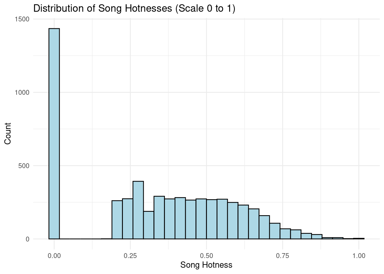
Exploring our research question, we want to understand the distribution of song hotness across all the songs.
music_tidy |>ggplot(mapping =aes(x = song_hotttnesss)) +geom_histogram(color ="black", fill ="lightblue") +labs(x ="Song Hotness",y ="Count",title ="Distribution of Song Hotnesses (Scale 0 to 1)" ) +theme_minimal()
`stat_bin()` using `bins = 30`. Pick better value with `binwidth`.
To see how song hotness relates to certain music genres, we want to find the top 10 genres with the highest mean rating of hotness. This will allow us to gain a better understanding of how genres affect listeners’ interest/appeal to songs.
# A tibble: 10 × 2
   artist_terms    mean_hotness
   <chr>                  <dbl>
 1 jam band               0.801
 2 merseybeat             0.746
 3 funky house            0.722
 4 speed metal            0.702
 5 space rock             0.691
 6 all-female             0.682
 7 rap rock               0.682
 8 hardcore techno        0.675
 9 piano rock             0.662
10 folk punk              0.661
We then explored how genre and song duration are related by identifying the mean song duration for each genre. In the future, we could potentially use this exploratory analysis to understand how song duration relates to the popularity or hotness of a song.
# A tibble: 402 × 2
   artist_terms                             mean_duration
   <chr>                                            <dbl>
 1 Russian Easter Festival_ Overture_ Op.36        22050
 2 protopunk                                         580.
 3 progressive rock                                  452.
 4 funk metal                                        440.
 5 space music                                       438.
 6 progressive trance                                427.
 7 dark ambient                                      426.
 8 techno                                            420.
 9 kizomba                                           413.
10 marimba                                           411.
# ℹ 392 more rows
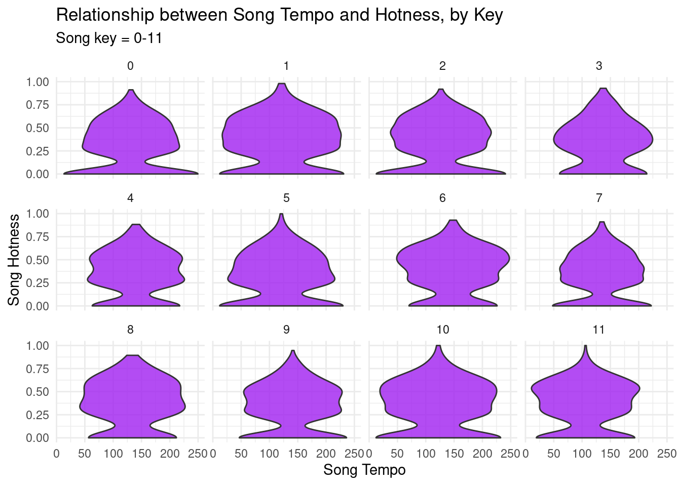
Lastly, we generated a violin-plot to describe the relationship between the variables song tempo and song hotness, and display these relationships separately by the key the song is in to make these plots more specific. We had to filter our tidied version of our dataset so that null values from the unclean original data-frame are not included in this plot. We wanted to explore the relationship between these variables to better understand how song tempo and hotness compare against each-other, while identifying how this relationship can change by the key of the song.
music_tidy_filtered <- music_tidy[music_tidy$song_key !="904.80281",] #cleaning cols for plotggplot(data = music_tidy_filtered, aes(x = song_tempo, y = song_hotttnesss)) +geom_violin(fill ="purple", alpha =0.8) +facet_wrap(~ song_key) +theme_minimal() +labs(x ="Song Tempo", y ="Song Hotness", title ="Relationship between Song Tempo and Hotness, by Key", subtitle ="Song key = 0-11")
Questions for reviewers
List specific questions for your peer reviewers and project mentor to answer in giving you feedback on this phase.
Which song characteristics do you think would be most interesting to compare to song hotness?
Do you think it would be beneficial to also explore the relationships between artists and artist popularity? Or to focus primarily on songs?
Are there any types of plots you think would (or wouldn’t) lend themselves well to data analysis on this dataset?