Harmonizing with Data: Exploring music through data science
Report
Introduction
Our group is most interested in researching the relationship between song characteristics (e.g. tempo, length, and loudness) and song popularity and whether or not certain song chatacteristics are more or less influential in this respect. We are using data from The Million Song Dataset, which was created in 2011. It contains information on artists (e.g.location, demographics, and popularity) and information on the artist’s respective songs (e.g. title, year, length, tempo, BPM, etc.).
Specifically, the research question we are looking to answer is “how do song characteristics like loudness, tempo, or length relate to song popularity (as measured by song_hotttnesss)?”
Based on our analysis, we found that song duration is not a statistically significant predictor of song popularity and that song loudness only has a small affect on song popularity.
Our hypothesis tests suggest that there is a statistically significant difference between the true mean popularity of slow vs. fast songs, but not between short vs. long songs.
Data description
Each row represents a song. The columns are:
artist.name: The name of the song’s artist.
artist.hotttnesss: A measure of the artist’s popularity, when downloaded (in Dec. 2010). Measured on a scale from 0 to 1.
artist.terms: The term (genre) most associated with this artist.
song.loudness: General loudness of the track.
song.tempo: Tempo in BPM.
song.duration: Duration of the track in seconds.
song.year: Year when this song was released.
song.hotttnesss: A measure of the song’s popularity, when downloaded (in Dec. 2010). Measured on a scale from 0 to 1.
song.key: Estimation of the key the song is in. Keys can be from 0 to 11.
song.time_signature: Time signature of the song, i.e. usual number of beats per bar.
num_songs: The number of songs an artist has in this dataset.
This dataset was created to derive data points about one million popular contemporary songs for use for machine learning and research related to music information retrieval algorithms at a commercial scale.
Echo Nest, LabROSA, and the National Science Foundation of America (NSF) funded the creation of the dataset.
Many variables, like song length and loudness, comes from objective statistics about songs, and therefore are unlikely to be biased or influenced by different processes. Song and artist “hotttnesss”, however, are likely to be influenced by 2010 social trends.
After downloading the CORGIS dataset, we grouped by artist name in order to count the number of songs each artist has, and then selected the variables that we thought would be interesting to compare against one another. We also removed NA values, but besides from this did not have to further tidy the data.
Since this data relates to music, people (music service users) are inherently involved. They likely were not aware of the data collection.
Data analysis
Data cleaning:
# A tibble: 4,214 × 11
# Groups:   artist_name [2,333]
   artist_name           artist_hotttnesss artist_terms song_loudness song_tempo
   <chr>                             <dbl> <chr>                <dbl>      <dbl>
 1 Casual                            0.402 hip hop             -11.2        92.2
 2 Gob                               0.402 pop punk             -4.50      130.
 3 Planet P Project                  0.332 new wave            -13.5        86.6
 4 Wayne Watson                      0.352 ccm                  -7.54      118.
 5 Blue Rodeo                        0.448 country rock         -8.58      120.
 6 Richard Souther                   0.331 chill-out           -16.1       128.
 7 Tesla                             0.513 hard rock            -5.27      150.
 8 Elena                             0.378 uk garage            -8.05      112.
 9 The Dillinger Escape…             0.542 math-core            -4.26      167.
10 SUE THOMPSON                      0.306 pop rock            -12.3       138.
# ℹ 4,204 more rows
# ℹ 6 more variables: song_duration <dbl>, song_year <int>,
#   song_hotttnesss <dbl>, song_key <dbl>, song_time_signature <dbl>,
#   num_songs <int>
We downloaded the music.csv dataset from the CORGIS website and imported it with read.csv(). Next, in order to create a column that has the number of songs in the dataset created by each artist, we grouped the rows by artist and used mutate() to add a column to the dataset that contained this number. After this, we filtered out the columns that we are not planning on using in our analysis. We decided to keep basic information about the artists like name, popularity, and genre. We also decided to keep columns that contained information about the songs’ characteristics like key, time signature, and duration. We also removed any songs with a song.hotttnesss value of zero or lower to focus our analysis on songs that achieved at least some popularity. Finally, we cleaned the column names and dropped any NA values in the dataset.
Summary statistics:
# A tibble: 1 × 8
  mean_loudness sd_loudness mean_duration sd_duration mean_tempo sd_tempo
          <dbl>       <dbl>         <dbl>       <dbl>      <dbl>    <dbl>
1         -9.56        5.04          241.        103.       125.     34.7
# ℹ 2 more variables: mean_hotness <dbl>, sd_hotness <dbl>
The average loudness of a song in the dataset is -9.56 with a standard deviation of 5.04. The average duration of the songs is 240.85 seconds, or about 4 minutes, with a standard deviation of 103.12 seconds. The average tempo of the sons is 124.52 beats per minute, with a standard deviation of 34.68 beats per minute. The average “hotttnesss” of the songs in the dataset is 0.459, with a standard deviation of 0.168. “Hotttnesss” is a measurement of song popularity that varies between 0 and 1.
Distribution of song hotttnesss
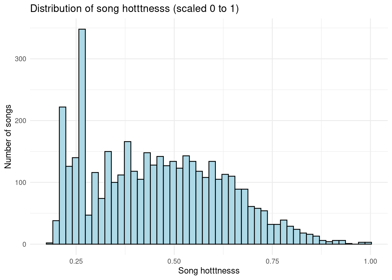
From this histogram, it is clear that the modal value of song hotttnesss is slightly above 0.25. The distribution appears unimodal and skewed right, with very few songs having hotttnesss values of 0.9 or above. Seeing how the modal value of song hotness is fairly low, this is ultimately why we would like to further explore why certain songs are much less or much more popular than others.
Distribution of song tempo
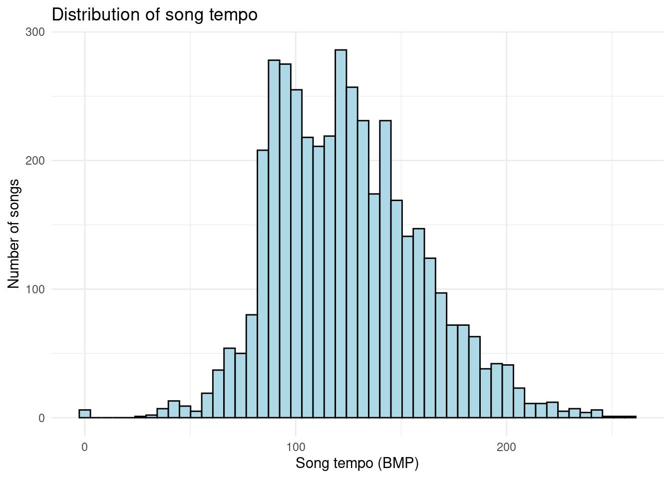
Looking at one of our key variables, we noticed that the distribution of song tempo appears bimodal. One peak appears slightly below 100 BPM and the other around 120 BPM. The tempos in the dataset appear to have a range of approximately 250.
Distribution of song loudness
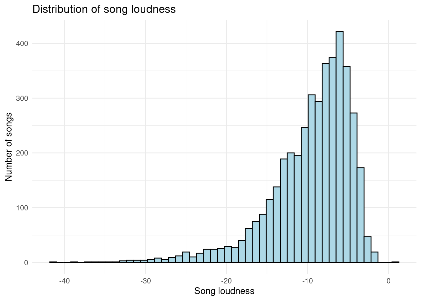
The distribution of song loudness in the dataset appears to be unimodal with a peak around -6 and is skewed left. Currently, it appears that a majority of songs have a high loudness, which is interesting to note because the distribution of song hotness was right skewed. We would like to better understand if there are any potential relationship between these two variables later on.
What is the relationship between song hotttnesss and song tempo?
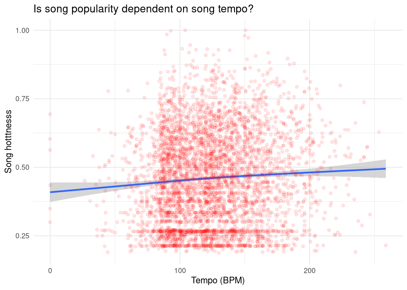
As we previously took note of song tempo distribution, we would like to observe how song tempo and hotness could be related. There appears to be almost no relationship between song hotttnesss and song tempo based on this model. However, it could be that there is a relationship between song hotttnesss and song tempo that exists only within certain music genres. To view this relationship, first we limited our analysis to the 11 most represented genres in the dataset, as these had at least 60 observations:
# A tibble: 11 × 2
   artist_terms     n
   <chr>        <int>
 1 blues-rock     207
 2 hip hop        167
 3 ccm             99
 4 post-grunge     95
 5 dance pop       70
 6 gangster rap    69
 7 country rock    68
 8 pop rock        64
 9 chanson         61
10 latin jazz      61
11 power pop       60
The most represented genres are blues-rock, hip hop, ccm, post-grunge, dance pop, gangster rap, country rock, pop rock, chanson, latin jazz, and power pop.
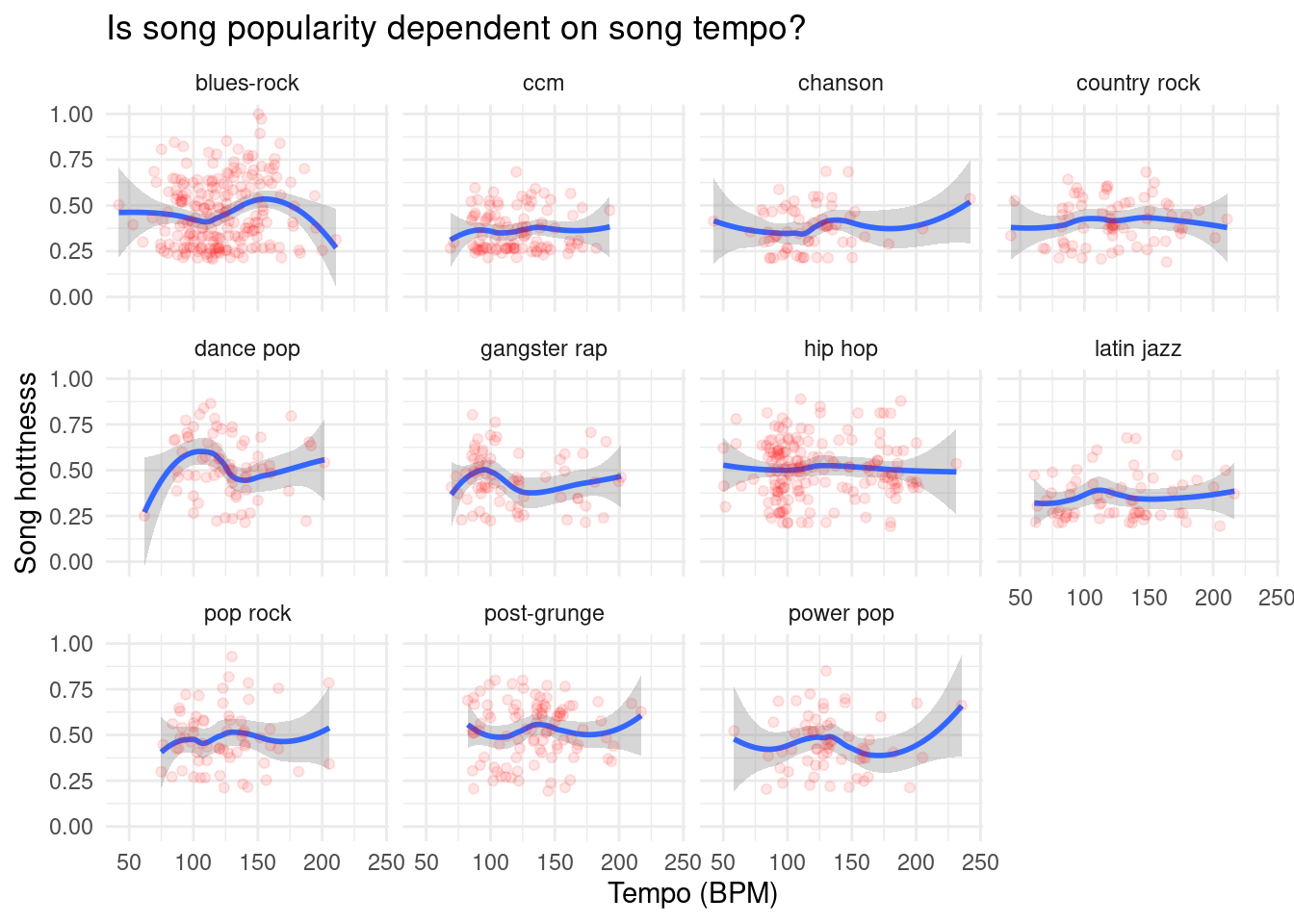
Even accounting for differences in genre, it still appears that there is no relationship between song tempo and song hotness. Perhaps it is difficult to observe a relationship by simply looking at these graphs, so we would like to still explore the relationship between song tempo and hotness through some linear regression models and hypothesis testing.
Can song hotttnesss be predicted with song duration?
# A tibble: 2 × 5
  term            estimate std.error statistic p.value
  <chr>              <dbl>     <dbl>     <dbl>   <dbl>
1 (Intercept)   0.459      0.00659     69.7      0
2 song_duration 0.00000226 0.0000251    0.0898   0.928
# A tibble: 1 × 12
r.squared adj.r.squared sigma statistic p.value df logLik AIC BIC
<dbl> <dbl> <dbl> <dbl> <dbl> <dbl> <dbl> <dbl> <dbl>
1 0.00000191 -0.000236 0.168 0.00806 0.928 1 1532. -3058. -3039.
# ℹ 3 more variables: deviance <dbl>, df.residual <int>, nobs <int>After analyzing a linear regression that predicts song hotness based on song duration, we found that the R-squared value is 0.000002. The adjusted R-squared value is -0.000236. This means that both the un-adjusted and adjusted amount of variability explained by the model is much less than 1%. Therefore, it appears that song duration is not a statisitcally significant predictor of song hotttnesss.
Can song hotttnesss be predicted with song loudness?
# A tibble: 2 × 5
  term          estimate std.error statistic  p.value
  <chr>            <dbl>     <dbl>     <dbl>    <dbl>
1 (Intercept)    0.527    0.00544       96.9 0
2 song_loudness  0.00704  0.000503      14.0 1.49e-43
# A tibble: 1 × 12
r.squared adj.r.squared sigma statistic p.value df logLik AIC BIC
<dbl> <dbl> <dbl> <dbl> <dbl> <dbl> <dbl> <dbl> <dbl>
1 0.0445 0.0442 0.164 196. 1.49e-43 1 1628. -3250. -3231.
# ℹ 3 more variables: deviance <dbl>, df.residual <int>, nobs <int>The R-squared value is 0.0445. The adjusted R-squared value is 0.0442. This means that both the un-adjusted and adjusted amount of variability explained by the model is approximately 4.4%. Therefore, it appears that song loudness is a better predictor of song hotttnesss than song duration is, but may overall not be the best predictor, as 4.4% is quite low.
\[ \widehat{hotttnesss} = 0.527 + 0.007 \times loudness \]
Regardless, we have written an equation for our linear regression model above. A song with 0 loudness is is expected to have a hotttnesss of 0.527. For every 1 unit increase in song loudness, we can expect song hotttnesss to increase by 0.007.
Evaluation of significance
Through our data analysis and modeling, we decided that we would still like to continue exploring how all three variables (song tempo, song duration, and song loudness) have an effect on song popularity.
Evaluation of the effect of song tempo on song popularity (as measured by song_hotttnesss)
Our group is interested in whether or not song popularity (measured by song_hotttnesss) is affected by tempo. In particular, we were curious if songs with a tempo faster than the median tempo (“fast” songs) have a statistically different mean popularity than songs with a tempo slower than the median tempo (“slow” songs).
Null Hypothesis: There is no difference between the mean popularity of slow songs and the mean popularity of fast songs. (0.343)
\[ H_0 : \mu_{slow} - \mu_{fast} = 0 \]
Alternative Hypothesis: There is a difference between the mean popularity of slow songs and the mean popularity of fast songs.
\[ H_A : \mu_{slow} - \mu_{fast} \neq 0 \]
# A tibble: 2 × 2
  speed mean_hotttnesss
  <chr>           <dbl>
1 fast            0.469
2 slow            0.449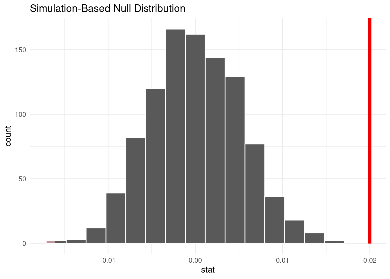
# A tibble: 1 × 1
  p_value
    <dbl>
1       0
Since the p-value (0.000) is smaller than 0.05, we reject the null hypothesis in favor of the alternative hypothesis. The data provides convincing evidence that the true mean popularity of fast songs is different than the true mean popularity of slow songs.
Evaluation of the effect of song length on song popularity (as measured by song_hotttnesss)
When completing our data analysis, we noticed the variation in song duration for different genres of music. As we recognize that different genres of music may have different song hotttnesss, we want to better understand patterns of song hotttnesss among songs of a long and short duration. To do this, we first find the median song duration in our dataset.
[1] 229.6159The median song duration is 229.62 seconds. We will use the median as the differentiating value between songs that are categorized as “long” vs. songs that are categorized as “short”. Songs longer than 229.62 seconds are long while songs that are 229.62 seconds or shorter are short. We would now like to see if there is an observable difference in song popularity for each of these groups.
# A tibble: 2 × 2
duration mean_hotttnesss
<chr> <dbl>
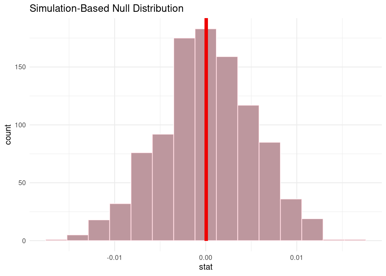
1 long 0.460
2 short 0.459We see that the mean song hotness/popularity of long and short songs are both 0.46. While there does not appear to be much of an observable difference, we want to better understand if there is a significant difference, so we will conduct a hypothesis test with the following null and alternative hypotheses.
Null hypothesis: There is no difference between the mean popularity of long songs and the mean popularity of short songs.
\[ H_0 : \mu_{long} - \mu_{short} = 0 \]
Alternative hypothesis: There is a difference between the mean popularity of long songs and the mean popularity of short songs.
\[ H_A : \mu_{long} - \mu_{short} \neq 0 \]
# A tibble: 1 × 1
  p_value
    <dbl>
1   0.986
Since the p-value (0.986) is larger then 0.05, we fail to reject the null hypothesis. Therefore, the data does not provide convincing evidence that the true mean popularity of long songs is different from the true mean popularity of short songs (i.e. we cannot prove they are different).
Evaluation of the effect of song loudness on song popularity (as measured by song_hotttnesss)
When completing our data analysis, we noticed that the distribution of song popularity and song loudness were inverse (song popularity was right skewed and song loudness was left skewed). We want to better understand patterns of song hotness among sounds of different loudness. To do this, we first find the median song loudness in our dataset.
[1] -8.4315The median general loudness of all tracks in our dataset is -8.43. With this median value, we will categorize songs louder than -8.43 as “loud” songs, while ones that are -8.43 or quieter will be “quiet”.
# A tibble: 2 × 2
loudness mean_hotttnesss
<chr> <dbl>
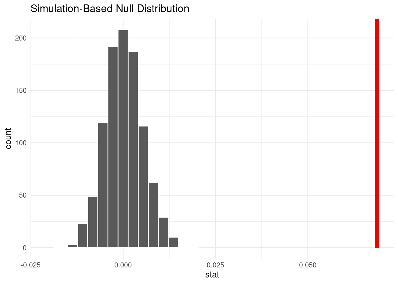
1 loud 0.494
2 quiet 0.425We see that the mean hotness of loud songs is 0.494, while that of quiet songs are 0.425. Here, we can see an observable difference between the mean hotness of different levels of loudness. So now to better understand this relationship, we would like to conduct a hypothesis test with the following null and alternative hypotheses.
Null hypothesis: There is no difference between the mean popularity of loud songs and the mean popularity of quiet songs.
\[ H_0 : \mu_{loud} - \mu_{quiet} = 0 \]
Alternative hypothesis: There is a difference between the mean popularity of long songs and the mean popularity of short songs.
\[ H_A : \mu_{loud} - \mu_{short} \neq 0 \]
# A tibble: 1 × 1
  p_value
    <dbl>
1       0
Since the p-value (0.000) is smaller than 0.05, we reject the null hypothesis in favor of the alternative hypothesis. The data provides convincing evidence that the true mean popularity of loud songs is different than the true mean popularity of quiet songs.
Interpretation and conclusions
The first relationship we analyzed was between song hotttnesss and tempo. We wanted to understand better if song popularity, or “hotttnesss”, was dependent on the tempo of the song. Our group wanted to look at the relationship between these two variables because we were divided by what tempos of songs we listen to, and wanted to better understand how the tempo of songs we like relates to the popularity of the song. We found almost no clear relationship between song hotttnesss and tempo, as the scatter plot was extremely spread out. This informs us that the popularity of a song from this dataset does not appear to be dependent on the tempo of the song.
However, after conducting a significant test to determine if songs with a faster than median tempo have a statistically significant different mean popularity than songs with a tempo slower than median tempo, the results were interesting. Our resulting p-value told us important information about the relationship between song tempo and popularity compared to the median tempo: Since our p-value of 0.000 is smaller than 5%, we reject the null hypothesis in favor of the alternative hypothesis. The data provides convincing evidence that the true mean popularity of fast songs is different than the true mean popularity of slow songs. Therefore, we were able to conclude that when dividing song tempos into “fast” vs “slow”, we were able to see that tempo levels did in fact have an effect on song popularity.
As seen in our data analysis section, we wondered if the reason for these differences in song popularity among fast and slow songs was dependent on genre. We considered the idea that certain genres may generally have faster tempos than other genres, so this could be the true underlying explanatory variable behind the differences in popularity. However, when observing song tempo and song popularity relationships through scatterplots and faceting by genre, the results of our stacked scatter plots show that there is no clear relationship between song tempo and hottnesss, even when separated by the 11 genres of this dataset. Ultimately, we were unsuccessful in determining a reason for why fast and slow songs may have different song popularity through data, but we can take a guess that perhaps song tempo can affect listeners’ mood, which would impact how they rate a song.
Next, we tested whether song duration could be used as a predictor for song popularity. After fitting a model using duration as the explanatory variable and song hotttnesss as the response variable, it was apparent that duration is not a good predictor for song hotttnesss based upon the adjusted R-squared value. To better understand why this was the case, our second significance test was completed looking at the effect of song duration on song popularity (song hotttnesss). After finding the median song duration of 229.61 seconds, we used this value as a differentiating value separating long and short songs. Our resulting p-value is 0.986 which is much larger than our boundary of 0.05, meaning that we will fail to reject the null hypothesis. This means that our results do not provide convincing evidence that the true mean long songs is different from the true mean popularity of short songs). These results can inform us that there is not sufficient evidence to disprove that the popularity of songs in our dataset differ by the length of the song. This makes sense that the popularity of songs can be found by a number of factors, and not purely by song length.
The last variable that we explored was song loudness; we tested whether song loudness could be used as a predictor for song popularity. We did this because we wondered if there was a relationship between songs that were very loud and songs that are very popular. Some members of our group greatly enjoy loud music, but wonder if this music is popular to others as well. Our results showed that for a 1 decibel increase in loudness of the song, we can expect song hotttnesss to increase by 0.007. Though this slope is very small, it is still positive, and paired with the significant adjusted R-squared value, we concluded that song loudness does have an affect on song hotttnesss. To further explore this relationship, we then conducted a third hypothesis test to determine the effect of song loudness on song popularity. We created two groups, “loud” songs vs “quiet” songs, which were differentiated by the median song loudness value. Through this test, we found a p value of very close to 0, which is lower than our significant value of 0.05. Because of this, we reject the null hypothesis in favor of the alternative hypothesis. The data provides convincing evidence that the true mean popularity of loud songs is different than the true mean popularity of quiet songs.
Ultimately, rom for further research and investigation on this topic could easily be diving more deeply into specific genres, artists, and decades of music.
Although there are a number of limitations with out dataset, as listed below, we are confident in our results. By interpreting the results of our data analysis in the context of real-life applications, we are better able to understand the relationship that we as college students have with listening to music. Each of our group members listens to music daily, making this project important to us in our daily lives. As each member of our group listens to different genres, artists, and decades of music, we represent a typical distribution of college students who listen to music daily. In the same way that each member of our group has different music tastes, so does the rest of the US. Due to the limitations of our dataset, we are not 100% able to unpack the relationships that a music listener has to their favorite songs, but we are able to draw meaningful conclusions as to what components might go into making a song with the most popularity.
Limitations
Our dataset includes some limitations. One problem is that not all songs have a year associated with them. Some songs have a year of 0, which would need to be dealt with in any analysis that involves time. Additionally, in the description of the variables for the Million Song Dataset on the Corgis Dataset Project website, song_hotttnesss is measured on a scale of 0 to 1. However, in the tibble, there are also negative values, such as -1. Furthermore, the song_key variable assigns numerical values to the different keys, instead of categorical values like “C major.” This makes it unclear what numerical value corresponds to which categorical value. This could be problematic if we did a data analysis using song_key, so we need to keep in mind that song_key maps a numerical value to a categorical one. Lastly, the definition of song_loudness is a bit abstract, as the website describes it as “general loudness of the track,” and these values are floats that are not on a specified scale / don’t have any meaningful units.
Additionally, while we can compare trends evident in this data, it is important to keep in mind that “how good” a song is is inherently biased, and that we are using the song_hotttnesss variable to be an approximate of that.
Acknowledgments
Thank you to the INFO 2950 course staff! Previous lectures and assignments were key to putting this report together.