Lab 3
Objective
The objective of this lab was to implement and test passive and active filters and compare them with what is theoretically predicted. One of the original goals was to implement and test a bandpass filter to be used on my robot in lab 4, though this goal was scrapped after I noticed its poor performance (as you will see as well).
Materials
- (1) robot from lab 2
- (2) LM358 op-amps
- (1) CMA-4544PF-W electret microphone
- (6) capacitors
- (13) resistors
- (10) M-M jumper wires
Process
Part 1
First, I simulated the behavior of simple passive lowpass and highpass filters using LTSpice, with R = 1.2 kOhm and C = 0.1 uF. Theoretically, the cutoff frequency for both filters using these component values should be 1326.3 Hz.
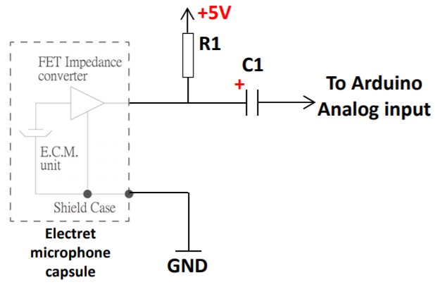
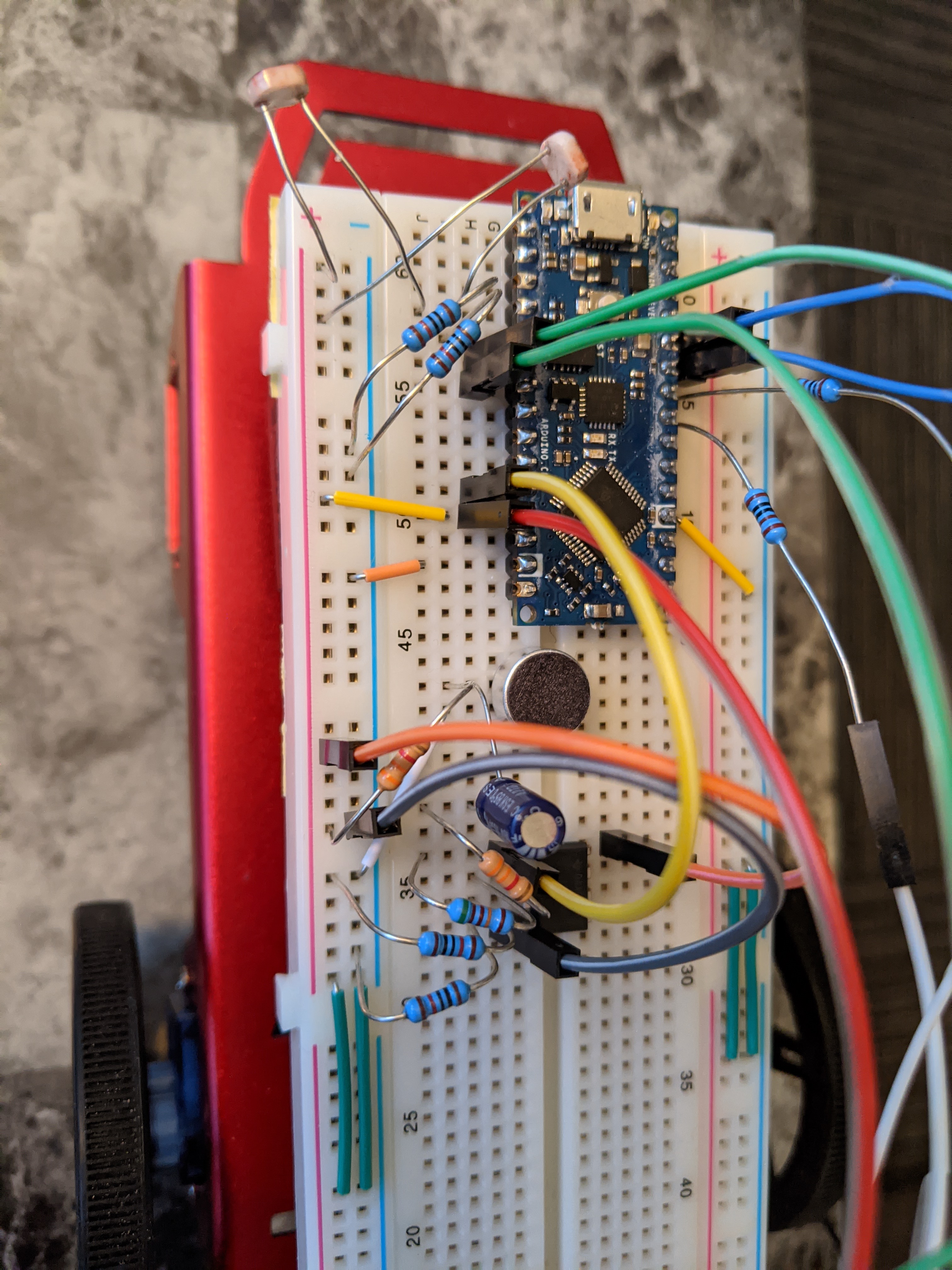
I next took a little detour and built the microphone circuit that would measure noises in the environment and connected the output to a pin on the Arduino Nano Every. This microphone circuit used an electret microphone along with one 3.3 kOhm resistor (R1) and one 10 uF capacitor (C1) according to the circuit diagram shown below.
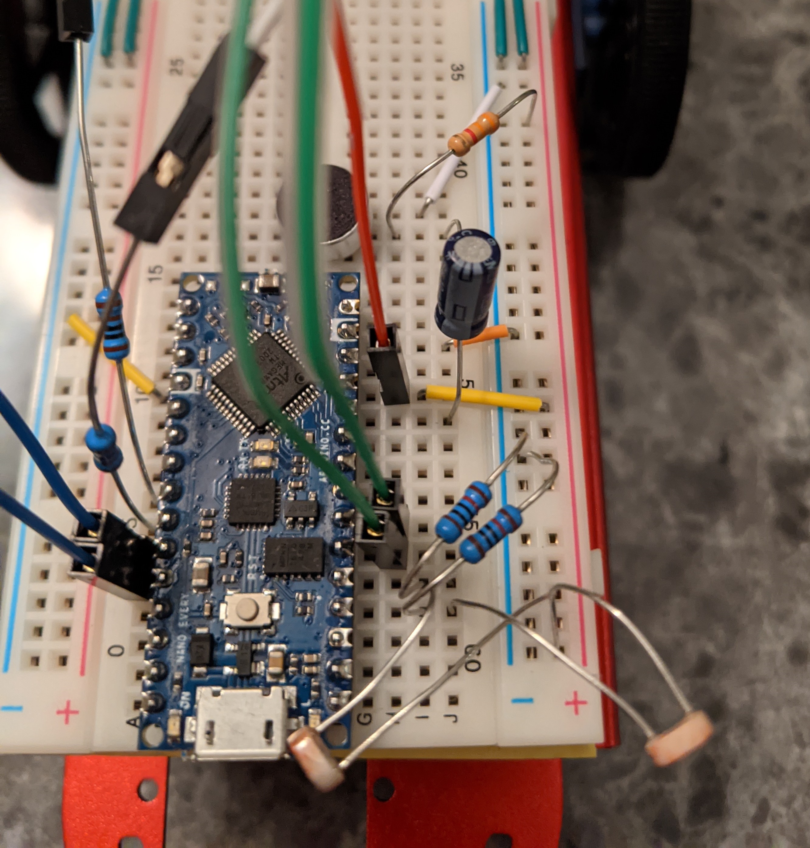
My breadboard looked like this, with the output of the circuit connected to pin A5 on the Nano Every.
The next step was to program the Nano to sample the microphone outputs and use MATLAB to perform Fourier analysis on those values in order to detect the dominant frequency of a sound. The analogRead() function is too slow for this purpose, so I manually set up the ADC in free-running mode by manipulating the appropriate bits in the appropriate AT4809 registers.
One nuance I encountered in this part was that the values from the ADC had to be converted from an unsigned 10 bit number to a signed 16 bit number. This is because even though sounds in the real world are comprised of sinusoids that oscillate between positive and negative values, the Arduino can't read negative values. The +5V supply is there to provide an offset so that the resulting waveform output from the microphone (i.e. ADC inputs) only has positive values. These values, which will now be between 0 and 1023, need to be shifted to be centered at 0 to more accurately reflect the real world values from which they were drawn, and scaled to 16 bit numbers (and printed to the serial monitor) for MATLAB to analyze.
The MATLAB code did three main tasks:
- play a sound or tone from my computer speakers
- collect the data printed to the serial monitor
- perform Fourier analysis (FFT) on the data
Note that the sampling frequency in this case is actually the frequency at which MATLAB fetches data from the serial port.
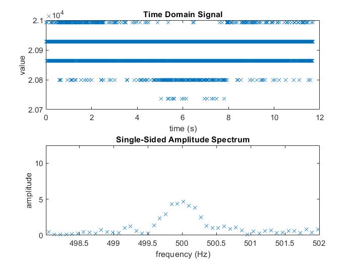
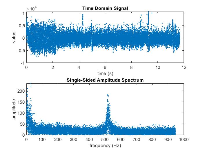
The time domain signal samples is plotted along with a zoomed in version of the Fourier amplitude graph that I obtained after playing a 500 Hz tone with this method is shown below.
Part 2
After noticing that the peak amplitude of the frequency spectrum was extremely small, I decided to improve the microphone circuit by amplifying the signal before feeding it to the Arduino.
To do this, I made a simple inverting amplifier using an op-amp with an offset into the V+ terminal. The circuit diagram is pictured below.
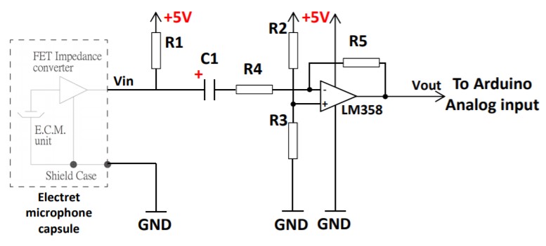
On my breadboard, the circuit looked as shown below. I used the same values for R1 and C1 as before, and used R2 = R3 = 10 kOhm, R4 = 3.3 kOhm, R5 = 511 kOhm. The theoretical output of this circuit is given by V_out = -V_in * R5/R4 + VCC/2.
The time domain signal and corresponding Fourier spectrum output from this circuit is graphed below.
Finally looping back to the lowpass and highpass circuits simulated at the beginning of Part 1, I built and tested them on my breadboard and analyzed the data using MATLAB after smoothing it. The plots that follow contain simulated and measured values for the transfer functions superimposed on the same graph after playing a 100 Hz to 1200 Hz sound over a 10 second duration. The first one is the lowpass transfer function; the second is the highpass transfer function.
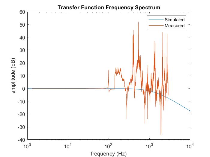
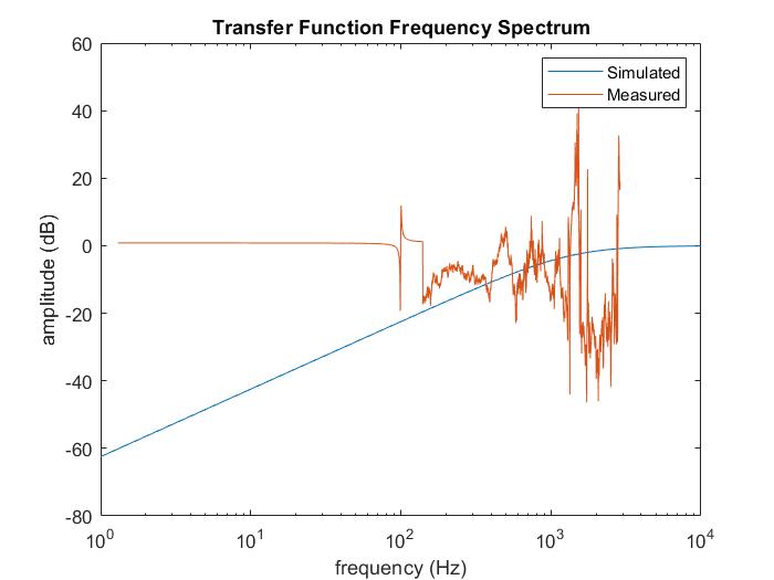
The plots show a clear deviation between experiemntal and theoretical data. This could be attributed to many reasons, from a noisy op amp to faulty components to a noisy environment and more. Luckily, this circuit will not be not used in the final robot.
I next tried to implement the Butterworth 4-pole active bandpass filter, which was chosen due to its flat frequency response and unity gain in the frequency range of interest, which is 500 Hz to 900 Hz in my case. The circuit diagram is pictured below.
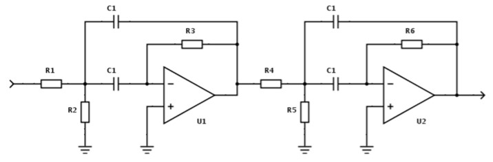
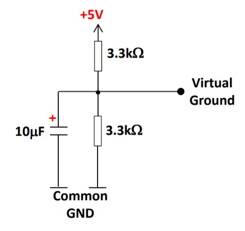
Note that the grounds in this circuit are actually virtual ground, providing a voltage offset to prevent op amp saturation. The schematic is shown below.
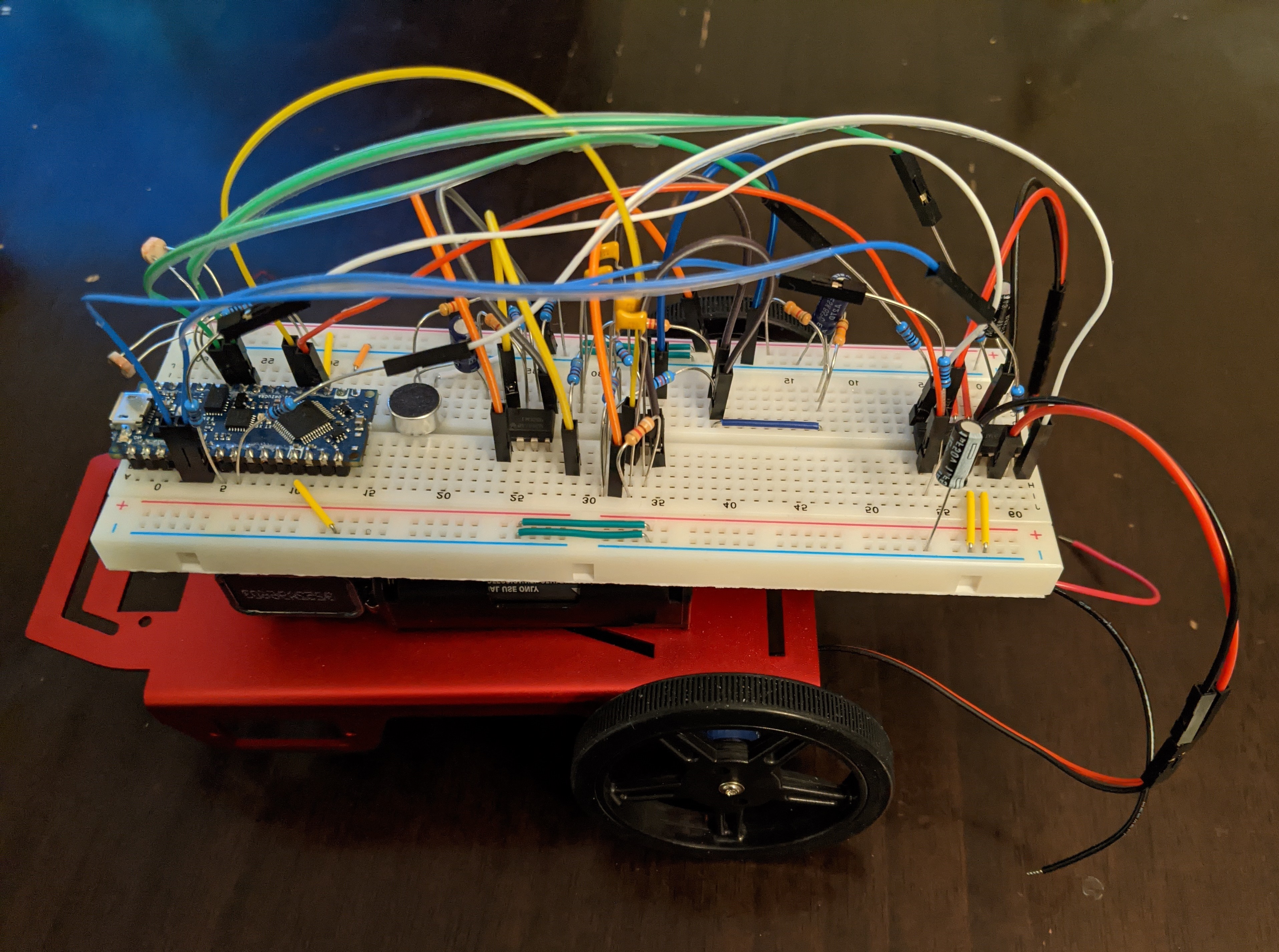
On my breadboard, the circuit looked as shown below. I used R1 = 4.87 kOhm, R2 = 620 ohm, R3 = 14 kOhm, R4 = 3.24 kOhm, R5 = 412 ohm, R6 = 9.1 kOhm and C1 = C2 = C3 = C4 = 0.1 uF.
The experimental frequency response for this circuit is plotted alongside the theoretical frequency response from LTSpice below.
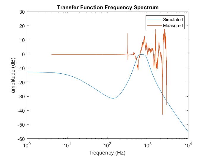
The shape of the band can be roughly seen between 700 Hz and 1020 Hz. There is still significant deviation between experimental and theoretical response, so in the end, I decided to take out the filter circuit entirely and connect the amplified signal directly to the Arduino pin.
Part 3
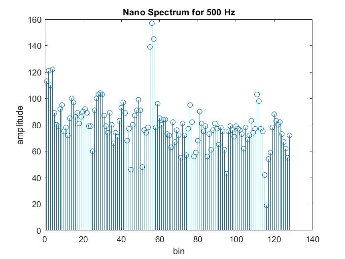
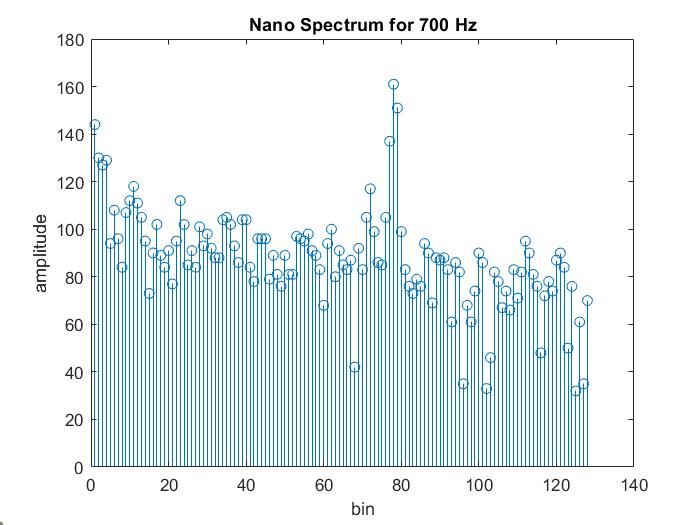
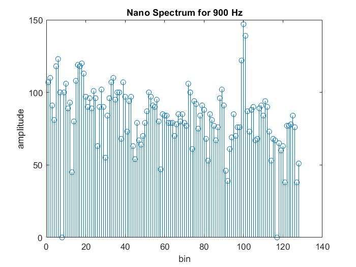
After removing the filter, all of the hardware was finalized for this lab. In terms of software, I shifted all Fourier analysis to be performed on the Arduino instead of MATLAB. To do this, I imported the Arduino FFT library, set up the ADC in free-running mode, and programmed TCA interrupts to sample pin A5 every 0.41667 ms (corresponding to a sampling frequency of 2400 Hz). I then took the 256-point FFT on the collected data, and used MATLAB to visualize the data, shown below for three different frequencies. Note that each bin (out of 128) corresponds to a range of frequencies, with the highest frequency being Fs/2 = 1200 Hz.
This concludes lab 3, which was primarily a foray into frequency analysis.
Next Steps
In Lab 4, I will be pulling everything I've done in this lab and previous labs together to make a robot that will be able to perform specific actions based on frequency that it detects.