Lab 3: Connecting and testing the Time-of-flight sensors.

The 2 time-of-flight sensors will be attatched to the sides of the robot. One sensor will be placed in front of the robot, and another will be placed in the back. The benefit of this is that the robot can see obstacles that can block forward motion, and easily reverse directions while keeping this ability. This does mean, however, that the robot can miss moving obstacles from either side, or anything on the ground.

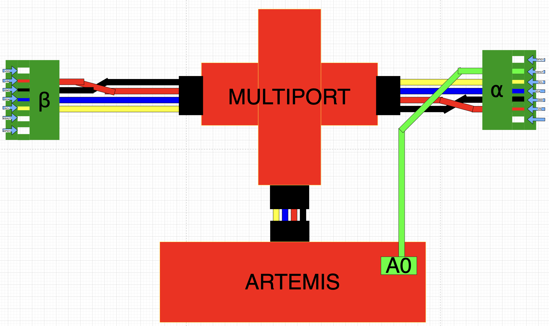
From the datasheet, it is noted that the I2C address for the sensors are both 0x52. This would be an issue for connecting both sensors simultaneously, however, unless one of the addresses is changed to something else. The method I chose was to connect one of the sensors to an Artemis output pin, call it the alpha sensor, shut it off by driving XSHUT low, assign a different address to the 2nd sensor, call it beta, then turn the alpha sensor back on. The image below shows the wiring setup for the sensors.

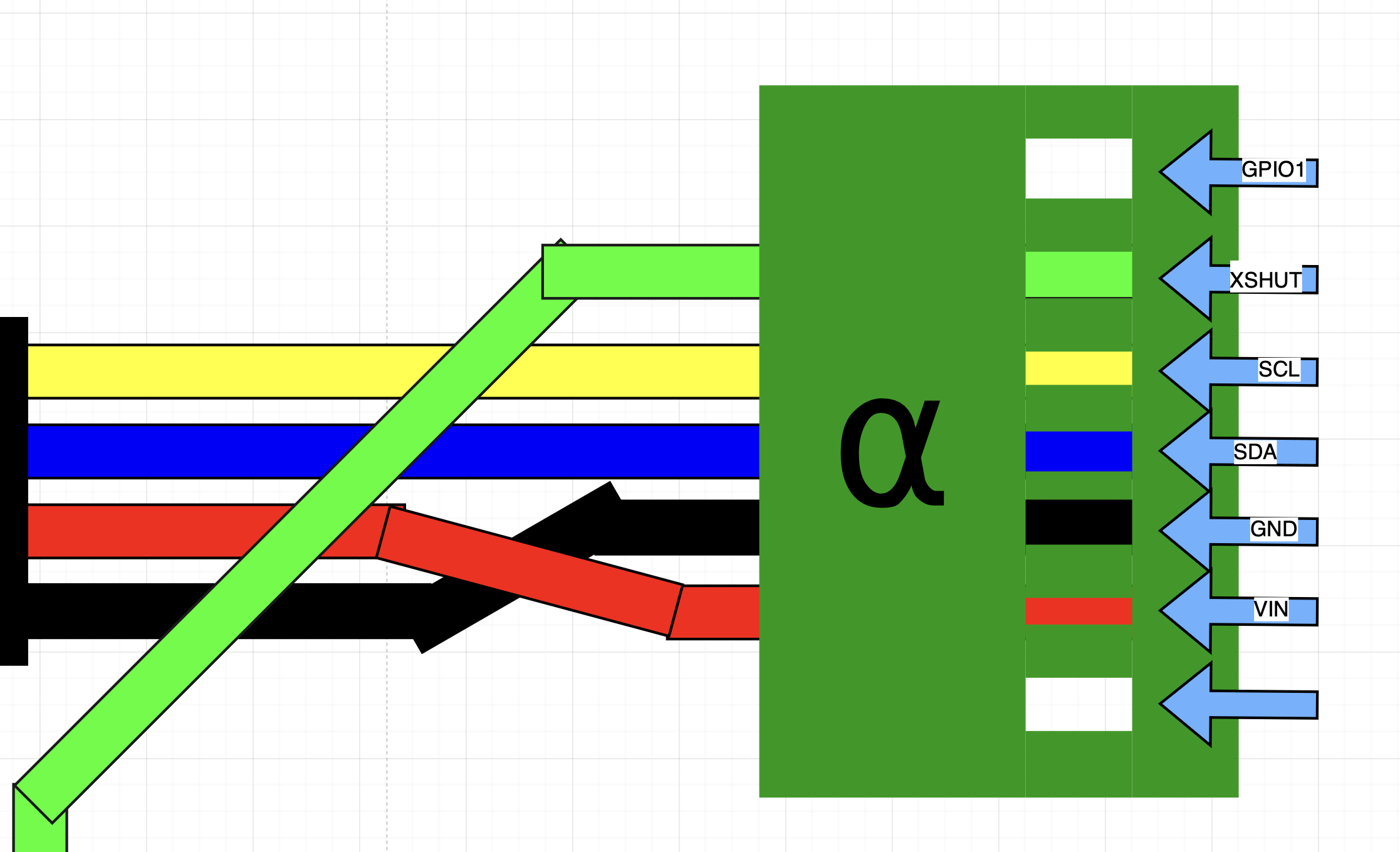
Zoomed in on the alpha sensor:

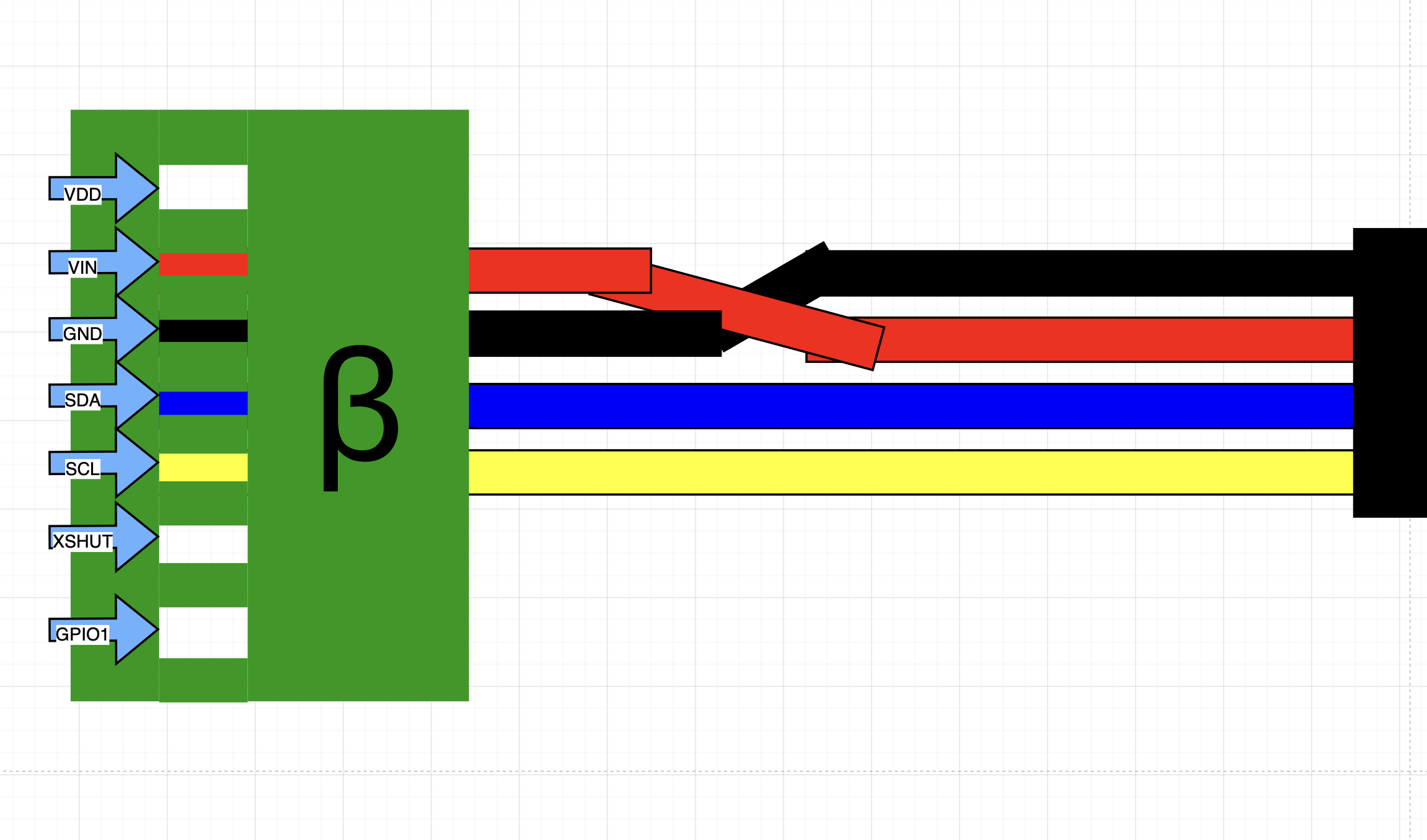
Then the beta sensor:

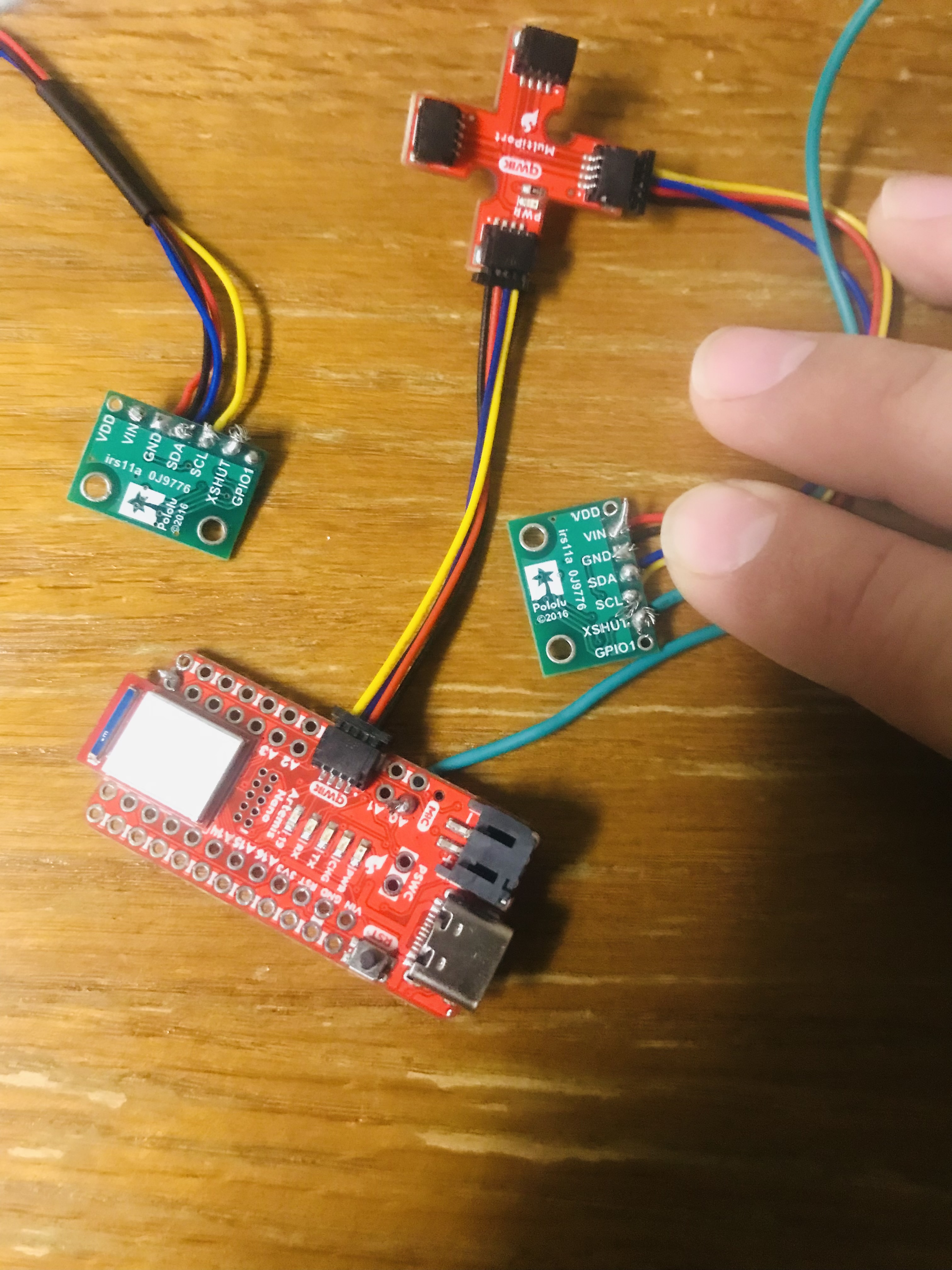
These connections were made partially using the QWIK connectors, then soldering the leads of one end to the sensors.

The alpha sensor was connected successfully as shown.

The Example code Example05_Wire_I2C.ino was then run on the Artemis to scan for I2C devices. It recognized the sensor, except at address 0x26 rather than the expected 0x52.

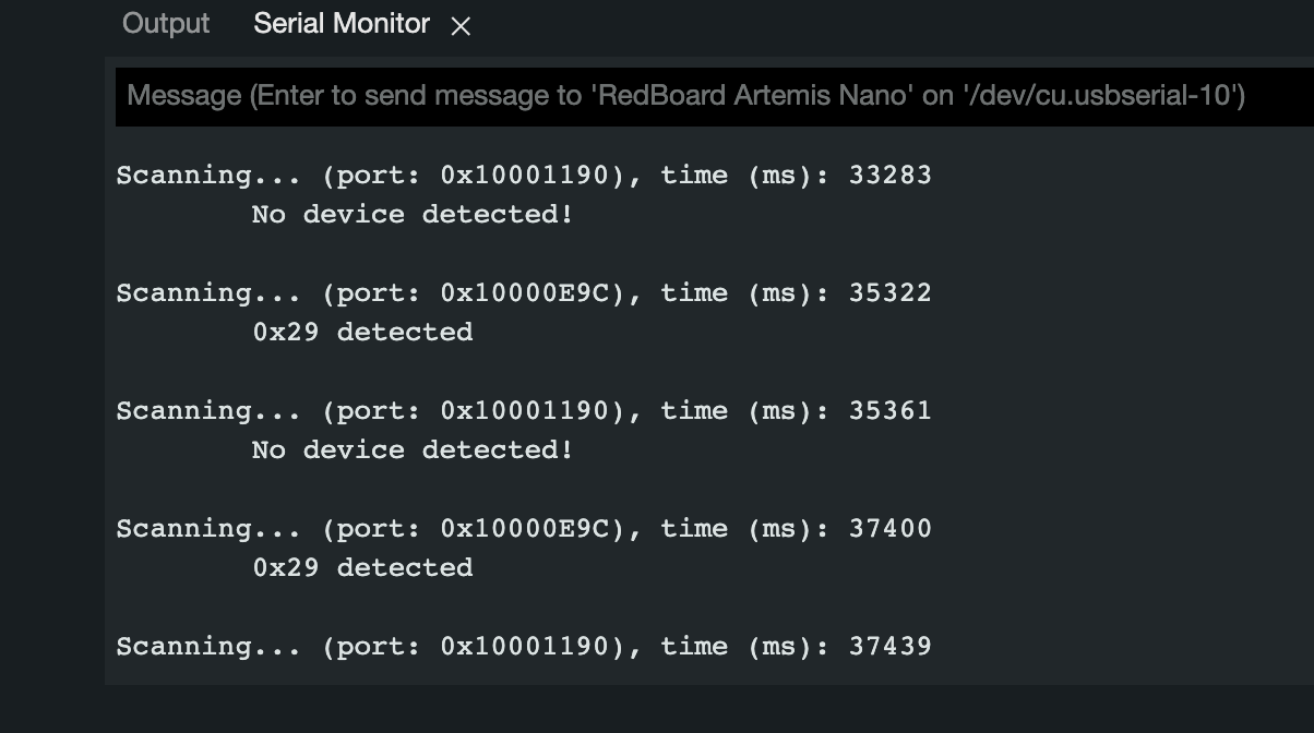
The difference in the addresses is 1 single bit shift; 0x26 is equal to 0x52 bitshifted to the right. This is due to the last bit in the address being reserved for whether the peripheral is being read or being written, according to the manual for the TOF sensor. The example code ignores this bit to form the address.

To get the two sensors working simultaneously, the alpha sensor was turned off, the beta sensor was changed to be address 0x54 (or kept at 0x2A, if there was a reboot), then the alpha sensor was brought back online, and accessible at its default address of 0x52.

Some care had to be taken in the code to ensure that it can work, even if the sensors maintain power during a reboot and the beta sensor retains its new address. After that was worked out, the alpha and beta sensors could be reliably measured and operated independently.

I decided that the long-range mode of the sensors would be most practical to use for the robot, considering it will be expected to navigate around a standard room, which are larger than 4m, and a larger range would be more desirable in this case.

To set up the testing environment, I modified the Lab 2 code for the Artemis by replacing the suite of callable functions, which each sent data over Bluetooth. I then collected this data on Jupyter Notebook to format into arrays of data containing measurements. I also included the TOFsensor.ino file, modified to use both sensors.

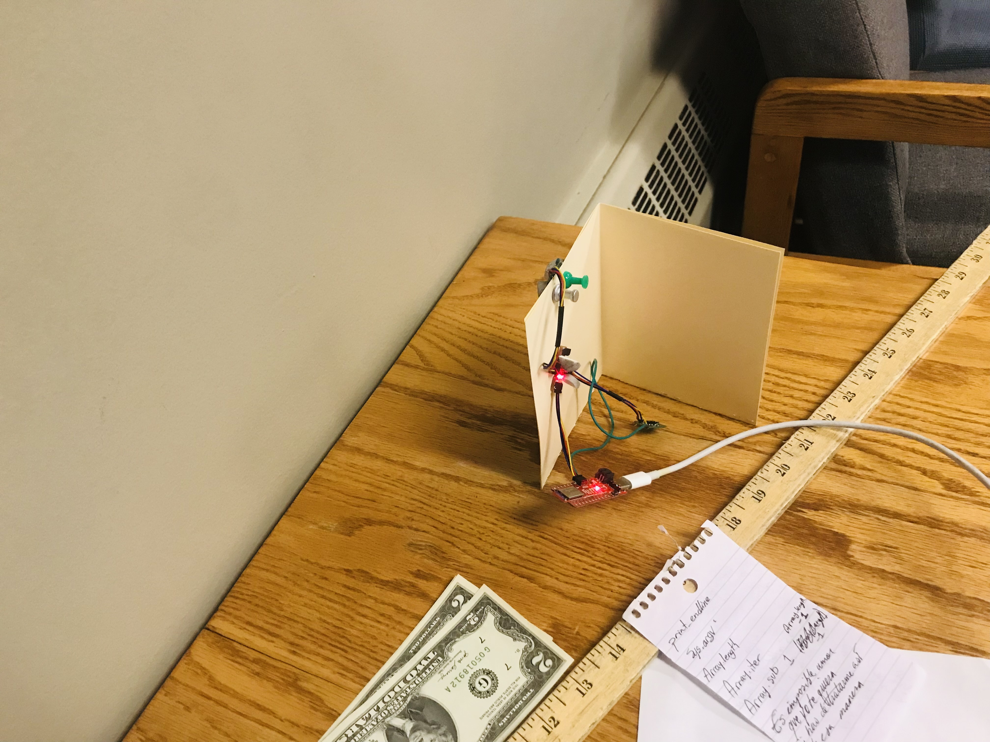
I decided to test the accuracy and range of the sensors. The Artemis was programmed to send a specified amount of data points on command from a single sensor, and the Jupyter Notebook processed the incoming string into an array of data points. A loop was set up to repeat this on command, allowing for the sensor to be moved into a known distance from the wall before taking data. Below is the setup used, where the beta sensor is facing the wall..

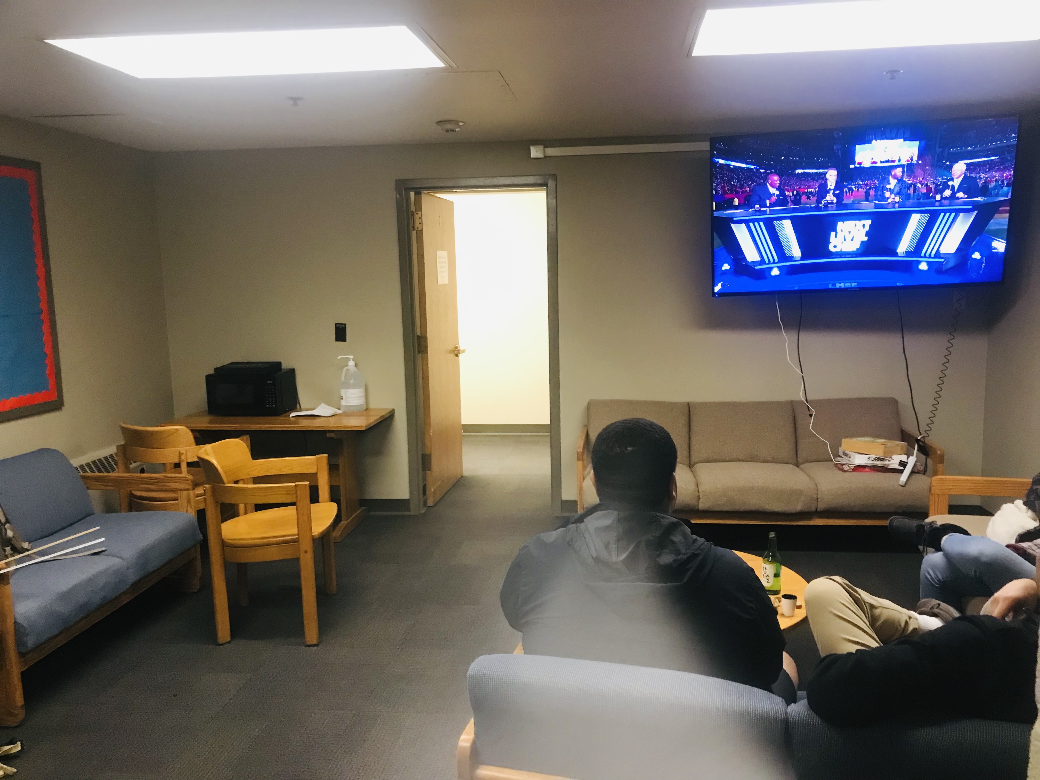
In a room like this.

The plot below is a scatter plot of the different distances measured vs. their actual distance. The measurement technique for the "actual" distance may be slightly innacurate, due to it relying on eyesight, but was useful in giving an understanding of the variation in sensor readings. Fifty data points were taken at each position from the wall.

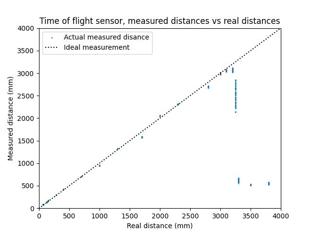
At 3.250m, the sensor behaves strangely, with a huge variation in readings. and seems to reach a much smaller value as distance increases from there. The range can be determined to be 3.100m, which is the last value read with reasonable accuracy.

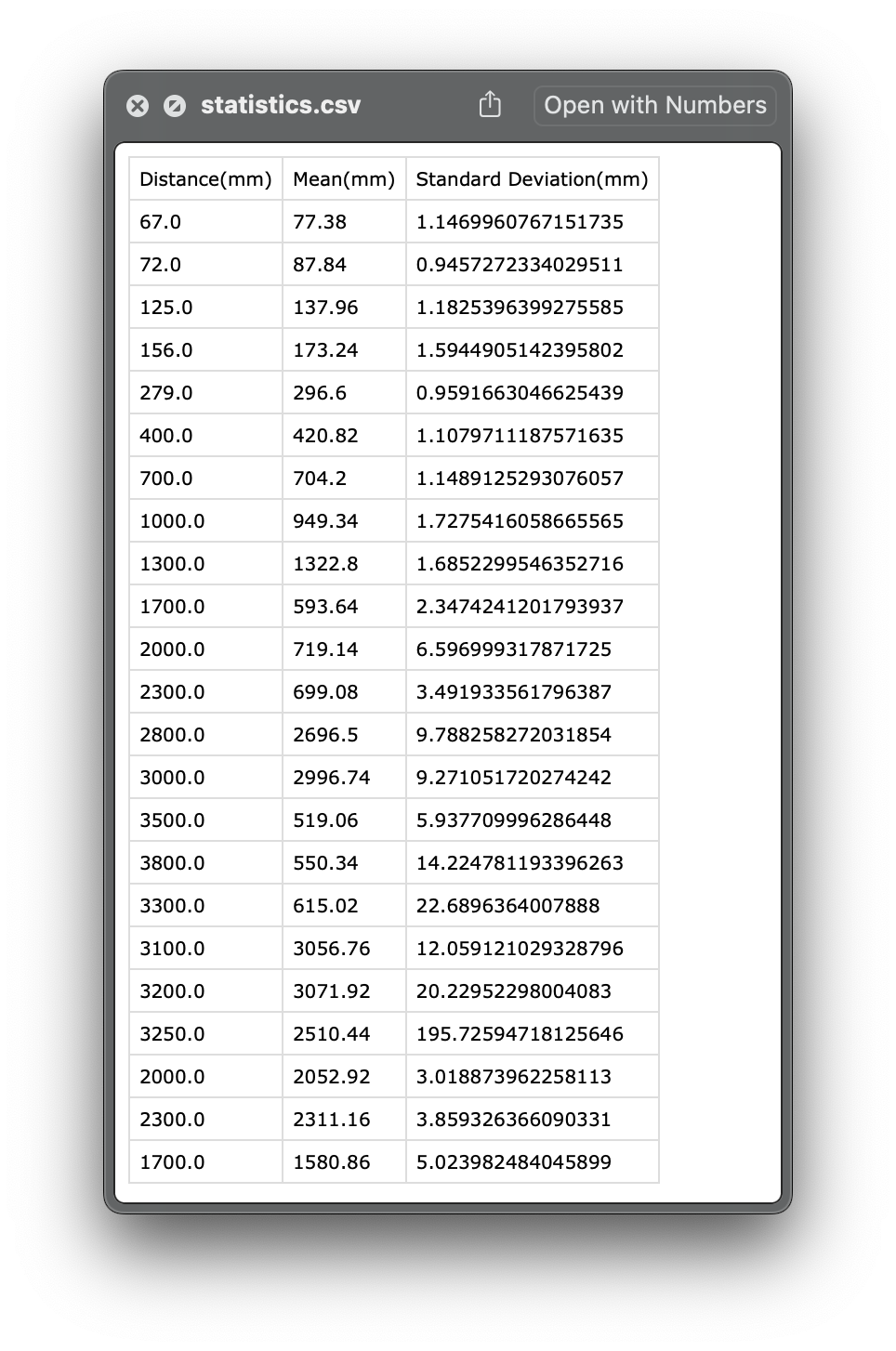
The sensor data also shows very little deviation from readings taken at the same place, meaning that average of the data may provide little no to increase in accuracy, so it would be unnecessary with the final robot.

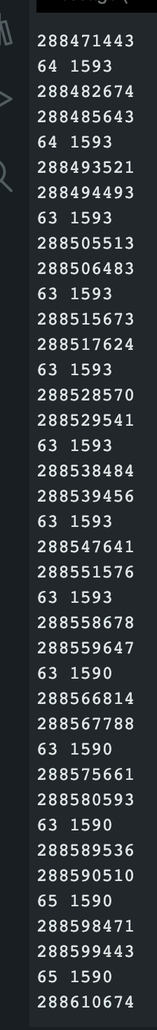
I added a function to the Artemis which would continuously print the time in microseconds until it receives sensor data, when it then prints the measured distance to the screen, for a specified amount of time.

The limitation of doing it this way is wasted time printing to the serial monitor: printing to the serial monitor takes a significant amount of time. With this in mind, the typical ranging time found this way was 9190us.

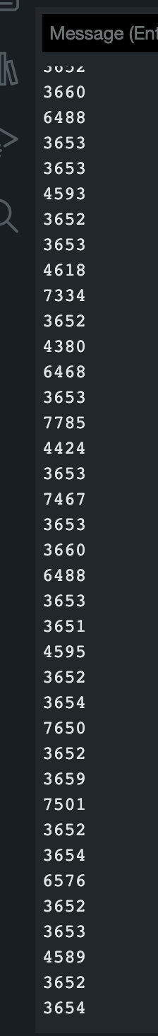
A new test was created to avoid this problem by only printing elapsed time to the serial monitor.

Which found the true delay to be closer to 3650us.

The lab was concluded by writing two functions. One for the Artemis, having it print out a formatted string, containing mutliple points of data, each containing a timestamp and a reading from each sensor. The other function was on Jupyter, which interpreted the string as a list of data. A successful trial run was performed, where the alpha sensor was kept a fixed distance from an obstruction, while the beta sensor had me waving a piece of paper in front of it slowly.

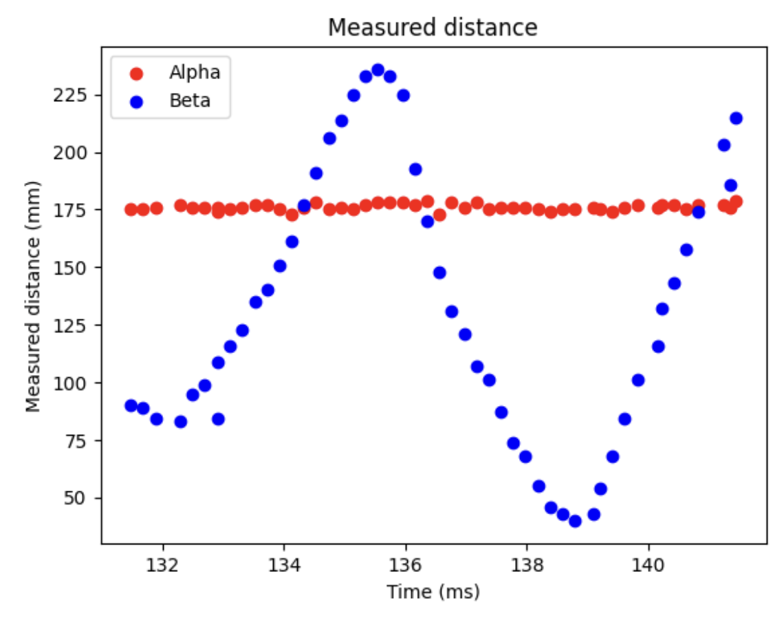
That's about it, really.