Lab 4: Recording IMU data.

Connecting the IMU was simple; the port leftover from the TOF sensors on the QWIK multiport adapter could be used directly. No address change was required, except for writing 1 to the AD0, since the LSB of the IMU address is determined by the logic level at AD0. After connecting the IMU, the example code "Example1_Basics" was ran to observe the data recorded by the IMU.

Moving the IMU around gave these results:

Action	Result
Move forward (+x)	ax↑
Move right (+y)	ay↑
Move up (+z)	az↑
Pitch up	gyr_y↓
Roll right	gyr_x↑
Yaw clockwise	gyr_z↑

Knowing this information, it was simple to calculate the pitch and roll from the accelerometer data.

Pitch	Roll
θ=tan-1(ax/az)	φ=tan-1(ay/az)

As a test, the pitch/roll at different orientations was found. The following image shows the setup, where the IMU was taped on top of a wooden block.

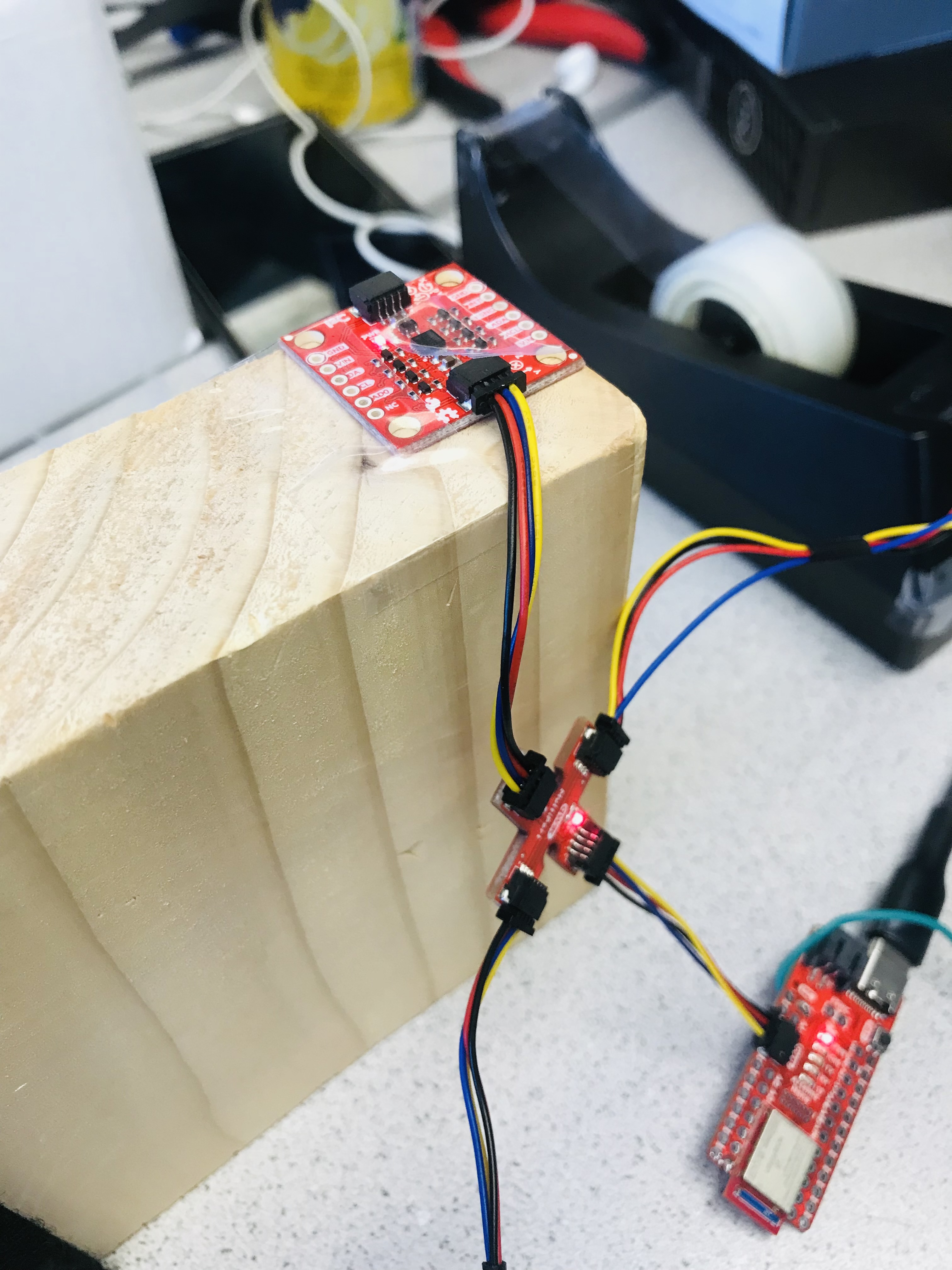
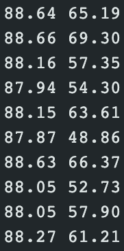
I rotated the block 90° forward, backward, right, and left to observe the effect on the IMU reading. The values in the table were gotten by averaging 10 data values. Before doing this, I noticed that at 90 degree angles, the z acceleration could get small enough to deviate from negative to positive, affecting the sign of the calculated angle. This was remedied by taking the absolute value of z if it was small enough.

Expectation	Pitch,°	Roll, °	STD in pitch, °	STD in roll, °	Image	Data (last 10 points averaged)
+90 Pitch	88.24	59.68	.2834	6.23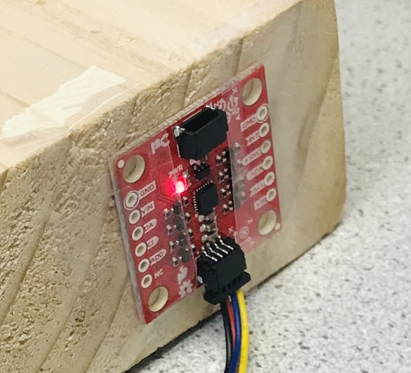
-90 Pitch	-89.35	24.96	0.412	39.5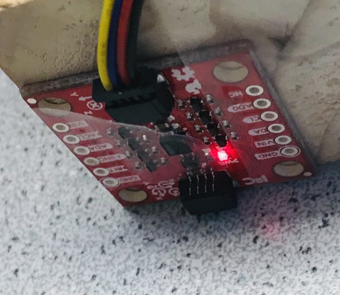
Plane, Zero	0.702	0.592	0.346	0.337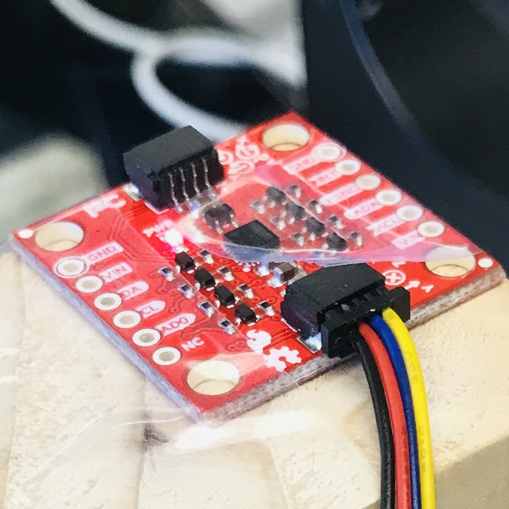
+90 Roll	70.63	89.67	16.2	0.232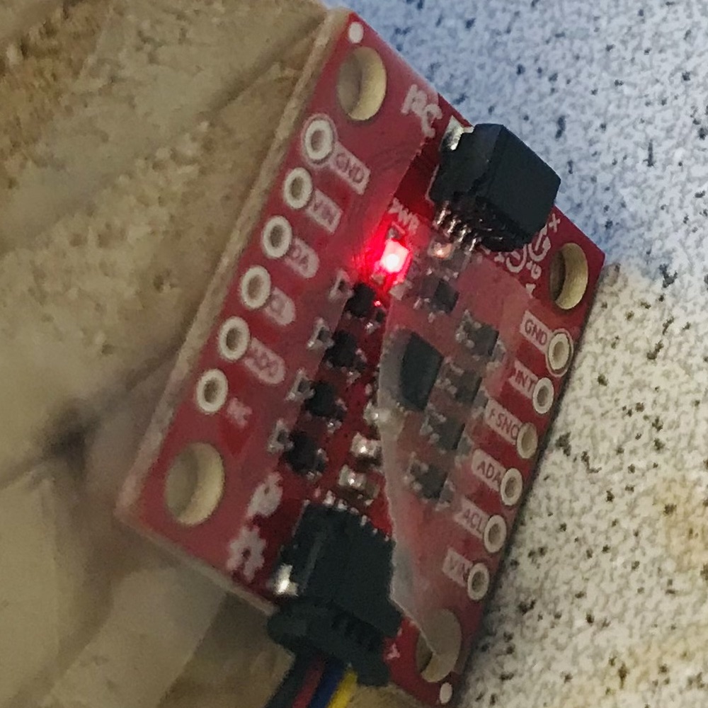
-90 Roll	48.47	-87.5	5.37	0.427	Image not taken :(

It's noticed that at these angles, one of either pitch/yaw is unable to be determined, with a large variation of measurements, around an incorrect mean. This is likely due to a_z and one of either a_x or a_y being very small, and hugely varying around zero. Otherise, the accelerometer seems to be fully accurate, being very close to the desired ±90 degrees that's desired. This suggests that the accelerometer data is unreliable for one of either pitch/roll at large angles.

Clean signals for acceleration, pitch and roll are desired. A fourier analysis on some data was taken to guide the design of the low pass filter. (The data was captured with the board on the robot.) Below is an image of the unfiltered acceleration data.

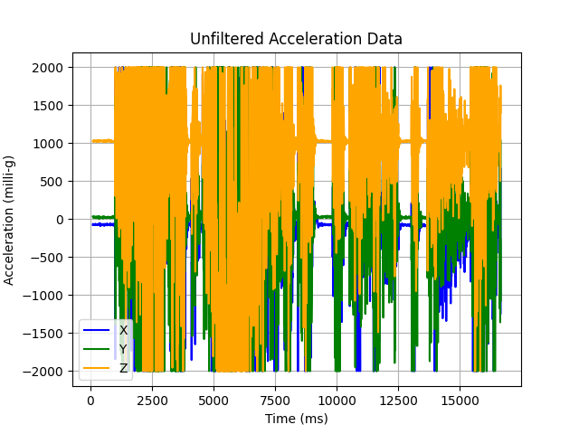
A fourier analysis of the data finds a large amoung of high-frequency noise is present in the signal.

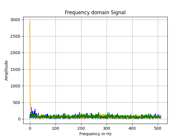
Below is the same data, but without having the z acceleration plotted

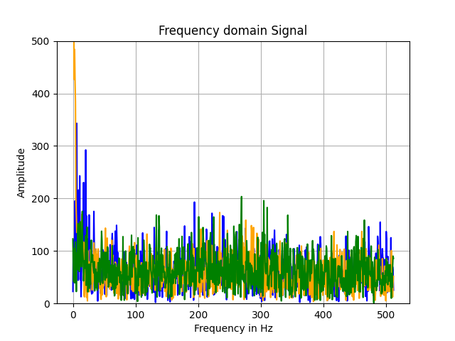
The desirable data is found in the <30 hertz range. The data was passed though a low pass filter @28.8Hz. The filtered data looks much more readable. The following is the filtered acceleration data, followed by the calculated pitch and roll.

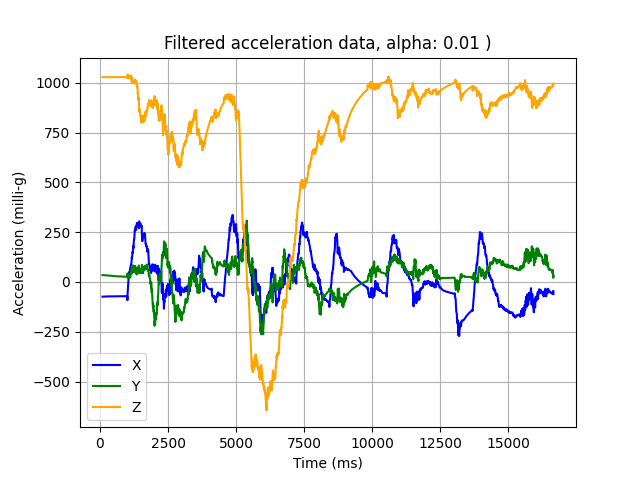
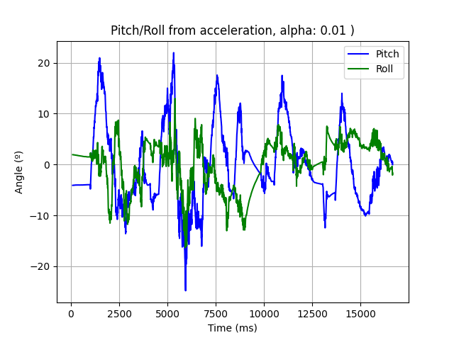
There was a significant improvement in the usability of the data. This data alone, however, serves only as a rough gauge of the IMU's position. To effectively determine the robot's position, the gyroscope will have to be used in conjunction with the accelerometer.

Before implementing the sensor fusion, the pitch, roll, and yaw were calculated using only the sensor data. A major difference is that the gyroscope data is cumulative change in angle, so angles greater than 180 are possible. To remedy this, a function was created to find an equivalent low angle.

Before taking data, a function on the board was written that would calculate the angle from the gyroscope data and continuously print to the serial monitor. As a test, the device was rotated in a similar manner to the accelerometer. The data was considered too unstable to reliably measure any angle, as the measured angle would have a heavy amount of drift, even at rest. One second the yaw is measured at 122°, the next at 117° For this reason the same {-90, 0, +90} degree tests were not performed as with the accelerometer. The following is a piece of the data where the sensor is sat perfectly still, and data is initialized at rest.

Drift was present even if the sensor was standing still; the measured changes in angles were all a small positive value, meaning that the overall angles in each direction were constantly increasing.

Gyroscope data taken during an RC car run was taken, then processed into the angular position. The results are below.

θn=Δθ * dt + θn-1

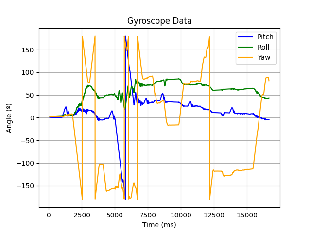
Drift is clearly visible, especially in the roll. To correct this drift, the gyroscope sensor data was fused with the accelerometer data. There were two factors used to correct the gyroscopic drift: 1 was a simple complementary filter with alpha = 0.1 (0.1 * acc data + 0.9 * gyr data) as well as a variable holding the amount of drift for each axis. This number is incremented/decremented whenever the gyroscope's measurement deviates from the accelerometer.

The result of the sensor fusion is low noise data with automatically correcting drift. The result is shown below.

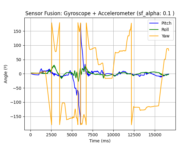
The drift correction was implemented because the simple partial filter wasn't enough. Say the gyroscope has drifted 50 degrees, while the accelerometer measures 0. Except for alpha=1.0, where acceleration data is given 100% of the weight, the measured angle will always be off. The tracked drift is programmed to slowly but surely eliminate drift over time. Careful choices were made to determine how fast, and when not to correct drift (ie., when the sensor is moving the most).

To gather data samples to make the above graph, I modified the code from lab 3 in a few ways. Instead of sending data samples as they're made, data collection was expedited by storing the data in an array first, then sending the array information over bluetooth. One big array contained time, accelerometer, gyroscope, and time-of-flight sensor data, was formatted to a string, and sent two at a time to the jupyter notebook. The string was then processed to a 2-D array, using spaces as column dividers and pipes as row dividers. After this is done, the data was processed using the low pass filter and sensor fusion as described above.

The video below shows some video captured during the data collection run used to make the previous graphs. During this run, 3000 data points were taken spanning 16.566s, for a sampling rate of 181.

The data collected is not the maximum that the board can store. The highest amount of data I can store before sending is 369404B (corresponding to 9000 data points, each 9 floats, each float 4B) which corresponds to about 45 seconds. However, longer data collection times increases the risk of having bluetooth disconnect. In that case it would be beneficial to have a seperate function to format the data and send it over bluetooth.

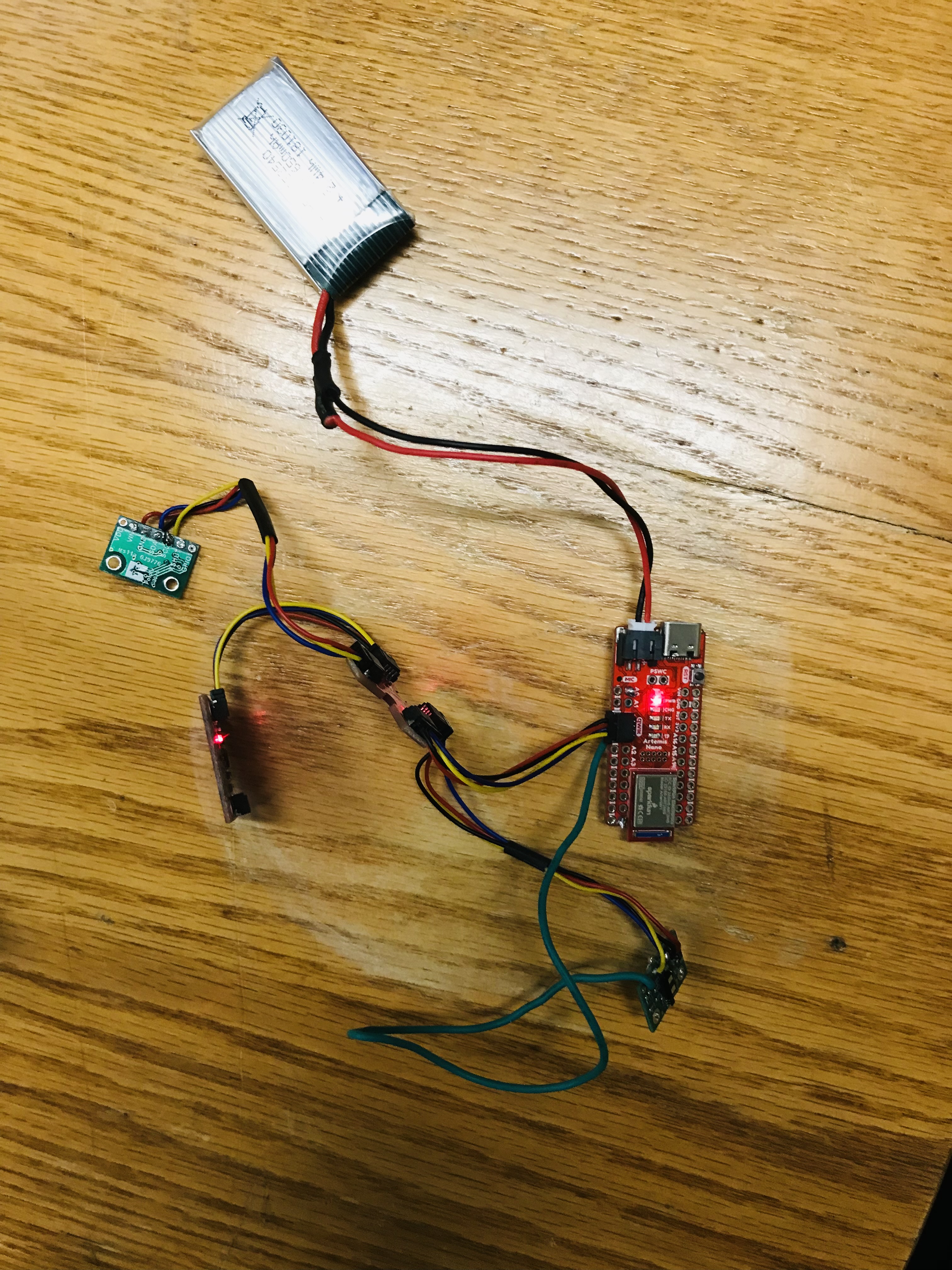
There were 3 supplied batteries to run the robot. They were all 3.7V lithium polymer batteries, offering the advantage of a large cycle capacity but with a lower capacity and longer charge time comapred to lithium ion. Two had capacity 650mA and one was 850mA. The higher capacity bettery ran the motors, and one of the lower capacity batteries was modified to connect to the board. Seperate batteries were used to eliminate noise in the power supply created by the motors, and the motors used the higher capacity battery since the board doesn't use much power, and a longer life is desired. Below is an image of the board connected to the battery.

Here's a recording of the RC car being controlled with its remote control.

Its movements are very abrupt, and the robot is difficult to control with position. The motion is jerky enough that a simple move-back followed by a move-forward will cause the car to flip. In future parts of the lab, it would be desirable to control the motors in a more nuanced manner.

In the video where data was taken (LINK), a complicated flip is seen. However, it can only be told from the calculated data that a simple 360° turn was made. This shows the limitations of the data collection method, as not enough detail is present to determine this from the data.

This is the end of this report. To go back home, click the... there's a button that takes you home, or something.