Lab 6: Using PID for orientation control.

Before beginning work on the PID controller, a system was set up to record and get data from the robot over bluetooth. This was done by storing float values to a 2-D array on the Arduino during operation, then iterating over the array and sending a set of data over bluetooth to a Jupyter Lab notebook on command. The code was reused from past labs to do this, but modified to send data values relevant specifically to PID control. The code below demonstrates the modification: the first 5 columns of the 2-D array are used to record relevant PID information, and the rest were ommitted. Strictly speaking, it was not necessary to include the funtion that created the whole array. This would've allowed for eliminating unused array space. However, as memory was not a limitation, the unused space was kept to allow for easy modification in the future.

And to send the data back, the floats were appending to the a string that would be sent over bluetoooth. To save characters on the string, floats that were "close enough" to ints were cast to ints before appending to the string (likely they were cast from ints to floats in the first place). It's not worth having a seperate int[][] and float[][] arrays to hold information: the Artemis uses the same amount of memory to store a float as it does an int. Loss of precision is not a concern, as the sensor readings don't exceed 6 digits of precision. This may be a problem in the future if more than ~100 seconds of data needs to be taken, as timestamps have millisecond precision, but this can be modified in the future if that much time is needed. The following code shows how data was sent back.

The string created by this code for each row was sent over bluetooh. The format was the following:

data1|data2|data3|...|dataN data1'|data2'...

Data rows (each corresponding to one point in time) were seperated by spaces, and data columns (each corresponding to a type of data) were seperated by '|'. The Jupyter notebook would then parse the strings into lists by seperating based on characters ' ' and '|'. The notification handler in the Jupyter notebook is set up to do this automatically and append each incoming data point to a big list of lists.

With the data side ready, I began work on the PID controller to maintain the robots orientation. This involved setting up a few functions on the Artemis.

First was a function that wrote a difference between the motor speeds. It takes a "difference" input and a "base speed" input, and the speed on the motors are adjusted so that the difference between the speeds equals "difference", a "difference" of 0 meant "base speed" was applied to both motors, and the motors were always assigned valid speeds (using 8 bit precision for PWM, this meant no more than a 100% duty cycle and no less than the duty cycle required for motion starting from rest, found in lab 5.). The minimum valid speed was increased, since turning motion was only possible at higher duty cycles. The following table shows some inputs to the function and it's outputs.

Input: difference	Input: base_speed	Output: motor 1	Output: motor 2
0	0	0	0
60	0	-30	30
200	0	-100	100
300	0	-100	100
0	10	10	10
10	20	10	30
60	20	-10	50

Motor speeds with different signs mean rotation. A speed of "1" is 1 + min_speed, the minimum speed that the motor should be run at to allow for rotation from rest. The maximum speed used the sample values in the table was 100 + min_speed, which is 255. In practice the minimum possible speed had to be increased to account for friction impeding the robot's rotation.

After this function was written, a PID function would simply need to pass a calculated "error" into the "difference", and have it's k constants adjusted for optimal performance. A loop was created that checked the IMU if new data was available, and if it was, would pass the gyroscope z (yaw) information to a PID function that returned a value that would be passed to "difference" in the previous function.

The "P" in PID stands for proportional. I wanted the speed difference between the motors to be proportional to the angular offset of the robot; if the robot is 10° off, the motors should be driven weaker than if at 50° off. The following formula, also used for lab 4.

Angle θ = gyrz * elapsedTime

Before implementing integration "I" or derivative "D" components to the PID controller, I got the following result by optimizing the proportionality constant.

This was a pretty good result, but I decided to add the "I" component (summing the error on each iteration) and the "D" components (an individual gyrz reading). I tuned these by iteratively increasing k_p, then k_i, then k_d, and each time stopping halfway between oscillations or underisable behavior occured. For rotation, it was important to keep speeds small, since the gyroscope had a limit to how much change in angle it could detect per reading. The following video is of the full PID controller in operation.

The orientation maintainence of the robot is improved, although it can be thrown off by extreme changes in angle. For the purposes of this lab, however, this can be accounted for and improved later.

After tuning the PID controller for orientation stability at rest, the controller was then tuned for stability in motion. A moderate speed was used for testing. A trial run using the same PID constants as at-rest control was done, and it was found that the controller was too weak to adjust the robot. The video below shows this under adjusted result.

The robot moves about 8° off course. This suggested that the same PID constants shouldn't be used for rotation vs. the forward motion of the robot. A new set of PID constants were created for the robot, which would be used only when the deviation in degrees is greater than a certain amount. The PID constants were gradually adjusted until the robot achieved a low deviation from on course. The video below is an example of an overshoot, where some undesirable oscillation is visible as a result of the controller being too sensitive.

A decent result was achieved by iteratively increasing the PID constants, in which the robot became 1.5' off course in the span of 30', a 2.5° error, an acceptable result given the drift of the gyroscope. Two such runs are shown below.

This result was acceptable given that the stunt is performed over 4 meters, ~12', so the drift will not be detrimental to operation.

The next phase was to combine the previous two results to pull of the stunt without any stop or pause:

1. Head towards a wall.
2. Once the robot is 1m away from the wall, do a 180° turn.
3. Head back to where the robot came.

In the PID loop, operations were performed in this order:

1. Poll IMU (if new data available, perform PID operation)
2. Poll front TOF sensor (if data available, reverse the robot if sensor reading is <1m)
3. Write timestamp, motor, last PID result, and last TOF reading to the array of data to send.

Reversing was performed by setting to 180° the amount of degrees the robot is off by. This lets the PID control adjust the robot to the right angle. A reverse done this way is shown at rest below.

Despite the video showing a decent turn of the robot, results were inconsistent, with the robot tending to overshoot the target angle. It was determined that the robot was turning too fast for the gyroscope, and maximum DPS (degrees per second) read by the sensor was increased fourfold. The result was a more consistent turning pattern, and the PID was retuned given this result. The video below shows a sample run of the robot on carpet performing the stunt.

The following video is referenced in reporting in lab 8. To go back there, click here.

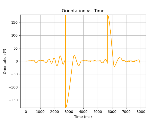
I then examed the data from this run as a test of the system. As expected, two clear turns are present. The turns are created by "injecting" a 180° error to the PID controller, which then completes a turn as it "corrects."

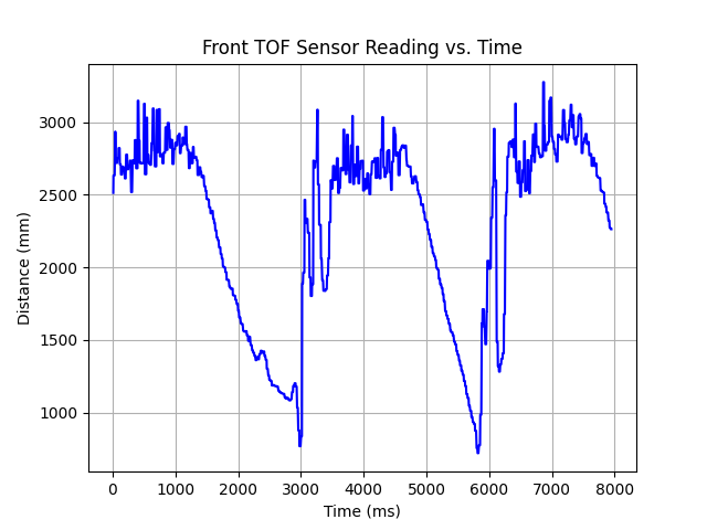
I then examined the sensor data. As expected, the reading was somewhat stable during durns and linearly decreased during forward motion. From the data it seems the robot was moving at 1.853 mps (4.14 mph).

I then repeated the runs on the floor in Phillips Hall. A problem that seemed to appear consistently is that the robot oscillated while coming out of the turn.

If you were sent from the lab 8 reporting, click here to go back.

There was another run where the robot was operated at a high speed. This led to it crashing into the wall, but was surprisingly able to recover well.

I made one more attempt at tuning the robot to remove oscillations. This involved changing the sign of the integration part of the PID controller to negative as well as reducing the cumulated error by a factor of 4 after each PID operation to avoid moving in the wrong direction. This change created great results, using the same P and I constants as before. The derivative part "D" wasn't needed and the k_d coefficient was set to 0. (UPDATE: See Lab 8 reporting for the improved PID calibration)

And finally, a test was performed running the robot at the maximum speed allowed by the PID controller, attemping to run as close as possible to the 100% duty cycle.

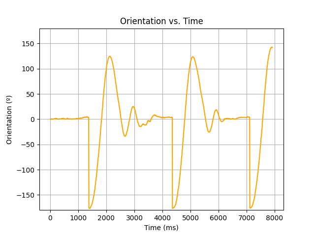
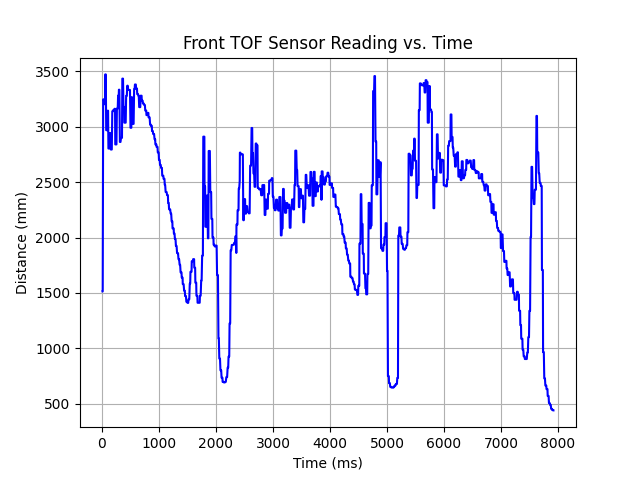
A limiting factor of the run was the time-of-flight sensor, as it was limited to a 50Hz refresh rate, even after optimizing the code and increasing the gyroscope's refresh rate. At high speeds this made it difficult for the robot to turn at exactly 1m from the wall. It was approximated here by setting the target distance to 1.7m, calibrated to turn the robot close to 1.0m. Below are graphs of the orientation and sensor readings over time.

The robot turns at about 750mm, which is pretty close to the target. The maximum speed observed from the data is about 3mps, 6.71mph. In conclusion, there remains to do a more precise way of getting the distance from the wall. For the purposes of this lab, however, calibrating it to be "close enough" will suffice.

This concludes reporting for lab 6. Click the button below to go home.