To build the Kalman filter, the steady-state speed and 90% rise time had to be found. A function was written the Artemis that would run the robot in a straight line (using PWM values used by the robot in a PID run when after moving straight) and collect time-of-flight sensor data continuously. The resulting graphs were gotten from this run.

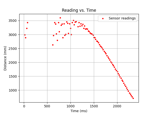
The graph above shows a shakiness when measuring at a large distance (>3m).

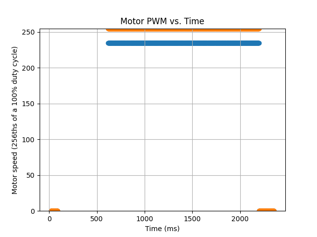
The blue data is the speed of the left motor, at 255, the highest PWM value in 8-bit. The orange data corresponds to the right motor, having a PWM value of 235, which balances out with the slower left motor to go straight.

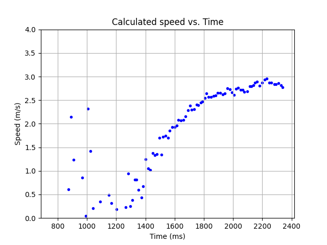
The robot was simply powered at the highest speed that would let it go straight, and it was found that the steady state speed was about 2.9/s. The speed was calculated by interpolating the sensor data, then applying a moving average function over every 10th data point. (Using a step size of 1 to represent 1ms, this corresponds to a d value of 1000ms/2900mm.) The time to rise to 90% of this steady state speed was determined to be 1.2s (therefore m would be d * 1.2/np.log(0.1)). On this basis the Kalman filter was built.

The Kalman function was built in the same way as it was introduced in class:

1. μ_p(t) = A * μ(t-1) + B * u(t)
2. Σ_p(t) = A * Σ(t-1) * A^T + Σ_u
3. K_KF = Σ_p(t) * C^T * ( C * Σ_p(t) * C^T + Σ_z)^-1
4. μ(t) = μ_p(t) + K_KF * ( z(t) - C * μ_p(t))
5. σ(t) = (I - K_KF * C) * Σ_p(t)
6. Return μ(t) and Σ(t)

This was implemented in Python using numpy functions. What remained was initializing the A, B, C, Σ_u and Σ_z arrays, as well as how the filter would be used. The C filter was set as [[1,0]], B was set as [[0],[1/m]], and A was set as [[0,1],[0,-d/m]]. The A and B arrays were then discretized using a Δt calculated by averaging the time between different sensor readings (as the sampling rate was increased on the sensor, the average time was 20ms, the minimum allowed by the sensor hardware.)

If want to go back to the lab 8 reporting, click here.

It was important that the filter have a high confidence in new sensor readings, but ignore sensor readings if they equal the last. The time of flight sensor may return a value despite not having a new value calculated by ranging, resulting in multiple "measurements" that are really just the result of a single measurement. Therefore the filter design must ignore equal sequential readings. Thus a distinction was made between "predicting" and "reading" using the Kalman filter.

A "read" will use a new unique sensor value and update the current state matrices (u and sigma) using a step size of the time since the last read.

A "prediction" will use the previous prediction/read for distance and predict the next state using the state matrices modified since the last read. The step size is equal to the time since the last read/prediction.

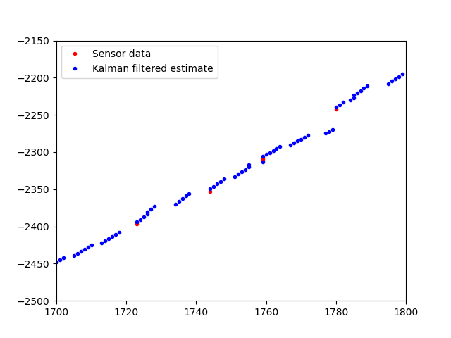
Predictions should never affect read values. This way the filter can make estimates of the current position of the robot without necessarily having a sensor reading to go off of. Some iterations of different starting variances/covariance matrices were tried before settling on the following standard deviations after one second: 20mm for sensor readings, 20mm for model distance, and 50mm/s for modelled velocity. The following result for the kalman filter after this process, which was satisfying.

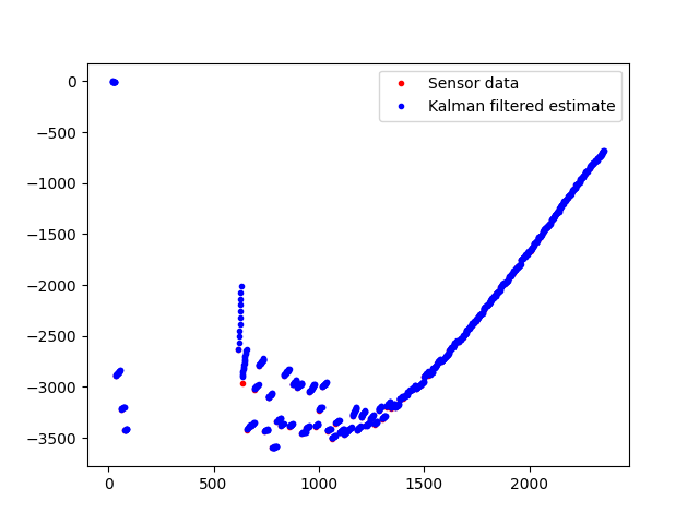
(Left axis, displacement from wall in mm. Bottom is time in ms). Below is a zoomed in image so you can appreciate the ability of the filter to "connect" sensor reading data points.

To expedite the stunt execution, I decided to implement the Klarman filter designed in Python on the robot. It was done in a similar manner to the python code, except that the current state of the robot was stored in a structure containing mu and sigma.

This is the return type for the Kalman function as constructed below.

This function was called by a read() or predict() function that uses the Kalman filter in different ways.

In the PID function that keeps orientation control, calls to KF::predict or KF::read are chosen based on whether new, unique data is available. The function includes debug statements used later prove the PID is working on the microcontroller.

The filter didn't work as expected the first time. Even after the code was debugged, the filter seemed to predict data points incorrectly, as seen in the below example of a failed run that used the Kalman filter while performing the stunt (stunt B, moving to the wall and turning back). The predicted data seems to go off of a calculated velocity that's too high.

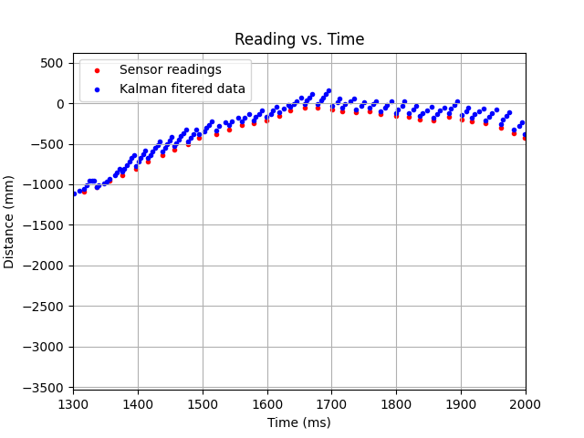
Some tinkering was done with the initialized values, and it was decided that the inital guess for d was off, where it should be a smaller 1000ms/4000mm. After this modification, the klarman filter results were found to be excellent as determining the robot's position. The following video shows a run used to test the efficacy of the kalman filter.

The following data was collected from this run, gotten by sending the stored information over bluetooth as was done in previous labs.

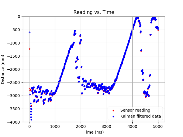
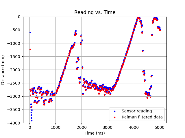
To appreciate the filter in action, here's a zoomed in graph at 1.4-1.8 seconds.

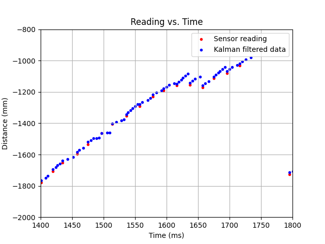
It's clear that simple linear interpolation couldn't produce results as good as the ones shown. For instance, at the data around 1650ms, the velocity that the Kalman filter goes off of changes to be less steep as the measured data points have an observed dip.

In conclusion, the Kalman filter is a useful tool to speed up operations and not have to wait for the data sensor to have new data. For execution of the stunt, it will be important to use this data in a meaningful way to predictably turn the robot in a precise spot; for the run, an earlier turning critereon (39") was used (instead of 24") since the current verision of the PID controlled turn is not able to turn the robot such that it has no forward momentem as the threshold (24"). In other words, the motors can engage in a turn at precisely the threshold, but that doesn't mean the robot won't continue moving forward with its momentum. This will have to be accounted for when speeding up the robot to its maximum speed for part 8 (it was operating slightly below maximum for the shown run). Also, below is proof the microcontroller is running the KF function running the debug version of the code shown previously (the debug code includes print statements).

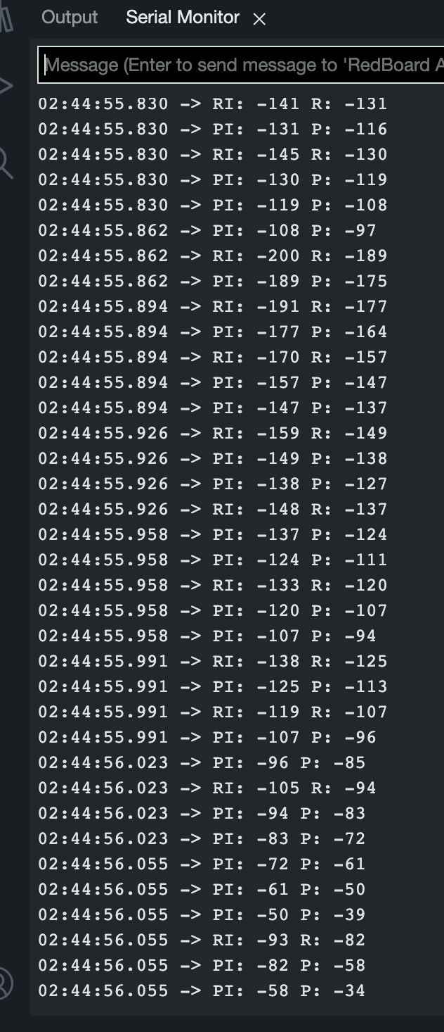
The image above shows the inputs/outputs of calls to predict "P" and read "R". As I wave my hand, the prediction tries to predict the next sensor reading, while the readings anchor the predictions to the expected value. I'm just waving my hand in front of the sensor to prove a point, so the sensor won't be able to predict accurately. But the Kalman filter is of course effective when the robot is in motion like was shown in the motor-powered run previously shown.