Chapter 18 Sample Allocation Model (SAM)

18.1 What is the Sample Allocation Model (SAM)?

The Sample Allocation Model (SAM) tries to identify an optimal surveillance strategy for areas with no observed cases of CWD, given the natural spread of the disease and the costs associated with surveillance.

The SAM framework provides 3 model settings that allow users to flexibly integrate the probability of disease spread with any historical sampling data and/or expense data to understand the probability that any given area presently has CWD, and thus how to best allocate a surveillance budget to be able to detect the introduction of CWD as early as possible.

This model is most appropriate for agencies where CWD has not yet been detected. An agency can still use this model if CWD has been detected, however, the positive sub-administrative units would have to be excluded therefore this model is not recommended if a large proportion of the state is positive.

18.2 What Questions Does it Answer?

Question 1. What is the probability that CWD has gone undetected given up to 3 years of historical sampling without finding a positive case? Model Mode 1 of SAM considers prior years of sampling along with the unobserved spread of CWD to determine the probability that any given sub-administrative area presently has CWD (i.e. posterior probability). Results can help reveal sub-administrative areas that may be “blind spots” in disease surveillance, where insufficient testing has occurred while CWD could be present and spreading silently. Alternatively, results can pinpoint sub-administrative areas where sampling has been sufficient through time such that CWD should have been detected by now if it were present. This model provides the probability that a sub-administrative unit presently has CWD and the probability that CWD prevalence is 1.0% or higher.

Note: To compute the probability of the freedom of disease after sampling has occurred, and given the clustering tendencies of hosts, use the Probability of Disease Freedom Using Clustering Model.

Question 2. Given the answer to Question 1, where should I look for CWD this coming year, and how much effort should I use given my agency’s CWD surveillance budget? Model Mode 2 of SAM builds on Model 1, utilizing the estimated probability of disease, a user-provided agency budget for disease surveillance, and costs per sample in each sub-administrative unit in order to strategically allocate a sampling plan over time across the entire agency. The resulting allocation constitutes the “optimal control” given a fixed surveillance budget. Optimal control means that the undetected spread of CWD across the jurisdiction is minimized at first detection, given the capped amount of sampling dollars available to make that first detection. In other words, optimal control is the best estimated balance of surveillance sampling under a budget to ensure that CWD is detected as early as possible. This model provides the same output as Model Mode 1 plus a state-level estimate of the total delay time between introduction and detection, and for each sub-administrative unit, recommended sampling sizes and corresponding probabilities of disease prevalence for multiple years (under the assumption that CWD remains undetected).

Question 3. Given the answers to Questions 1-2, what budget can improve this year’s surveillance program (i.e., reduce silent spread up to the moment of first detection)? Model Mode 3 builds on Models 1 and 2 to further consider how optimal control may change given a smaller or larger budget than an agency’s current budget. This model optimizes sampling strategies over various budgets to identify the best way to achieve earlier detection and more strategic allocation relative to current practices, minimizing cost while maintaining sufficient sampling. This model provides the same output as Model Modes 1 and 2, plus a cost analysis that demonstrates how optimal control changes given different budgets, which will be helpful for planning the annual budget necessary to bolster an agency’s surveillance program.

Note: SAM produces surveillance targets based on sampling optimization over a budget. It does not, however, produce standard errors or statistical confidence. To determine sample sizes necessary to reach statistical assurance that CWD is absent in an area, refer to the Sample Size Quotas Using Clustering Model or the Efficient Sample Size Calculator.

18.3 Abbreviated Tutorial

Part of the input required for SAM includes output from a previously executed Risk-weighted Surveillance Quotas model. Before running SAM, ensure there has been a “Risk” model executed for use in SAM.
Run the Sample Allocation Model (SAM) from the CWD Data Warehouse.
Select model Mode:
- Explore probabilities of disease status (Mode 1).
- Explore probabilities of disease status and obtain surveillance sampling targets (Mode 2).
- Explore probabilities of disease status, obtain surveillance sampling targets, and run the cost analysis (Mode 3).
Provide other necessary inputs: target season-year, number of years of historical data to be used (i.e. number of years before target season-year), annual growth rate, agency budget, per-sample costs, and maximum sampling capacity.
Specify Risk model to be used in SAM model.
Explore the model logs, input file, and output files from the model execution.
Explore the visualizations from the model execution.
If the model did not run, check the model logs to understand required data that was missing.

18.4 Parameters Needed to Execute the Model

Model type: Select ‘Sample Allocation Model (SAM)’ from the drop-down list.
Reference name: Label the model execution.
Applicable season-year (Optional): Label the season-year of the run to assist in documentation.
Notes (Optional): Enter any remarks about the model execution.
Mode:

Select Mode 1 to: Determine the probability that CWD has gone undetected (i.e., answer Question 1). [Shortest runtime]

Select Mode 2 to: Determine the probability that CWD has gone undetected then allocate a sampling plan (i.e., answer Question 2). [Moderate runtime]

Select Mode 3 to: Determine the probability that CWD has gone undetected, allocate a sampling plan, then conduct a cost analysis to further improve optimal control (i.e., answer question 3). [Longest runtime]
Season-year: The target season-year for which to plan for, this should be the upcoming (or future) season-year.
Total budget: The total annual budget that can be spent on CWD surveillance across the whole agency in the upcoming season-year. Not required for Model 1.
Look-back period: SAM can be used to compute the probability of disease presence using 0-3 prior years of historical negative sampling data. Any sub-administrative units that have historical positive results should be excluded from the model.

Look-back period of 0 years: Model will assume all sub-administrative areas are presently disease free; results will show 0% chance of current CWD presence in any sub-administrative unit.

Look-back period of 1 to 3 years: Model will use 1-3 years of data to compute the probability of disease presence based on the prior year(s) of negative sampling data. Any sub-administrative units that did not have any sampling in the look back period will have historical sampling values set to 0. Similarly, when the look-back period goes back further than available data it will be assumed that no sampling took place, i.e. historical samples equal 0. For example, if the target season year is 2025-26 and 3 years of look back are specified in an agency with data only from 2024-25, the model will use 2024-25 as historical year 1, and 2023-24 and 2022-23 will be included as historical year 2 and 3 - as specified - but they will be filled with 0s to indicate no sampling took place.

Note: Look-back period is limited to 3 historical years because SAM assumes that the introduction risk is static. Changes in introduction risk include new CWD outbreaks in neighboring areas, additional avenues of anthropogenic prion introduction, etc.
Annual growth rate: The rate that governs the annual increase in CWD prevalence (once established) in a region. This is a number between 0 and 1, where larger values correspond to faster spread of the disease. The default value is 0.2, which reflects the rise in prevalence from 0.5% to 1% over approximately five to seven years [1].
Risk model: The results of a previously executed Risk-weight Surveillance Quotas model for the agency (applicable for the target season-year). Note, any sub-administrative areas that have no risk, i.e. resulting quota of 0, should be excluded from the model (note, the model error log will indicate which sub-administrative units should be excluded ).
For each sub-administrative unit:
- Include: A check box to indicate which sub-administrative units should be included in the model, i.e. the sub-administrative units where sampling will take place. Sub-administrative units where CWD has already been detected should be excluded.
- Expense: The per-sample cost of surveillance in that sub-administrative unit (e.g. a single, sample-level cost that incorporates all costs of testing, such as equipment, personnel time, procurement, etc.). An expense is required for each included sub-administrative unit.
  
  Note, this model will later be incorporated with the Per-Sample Cost Analysis model where per-sample costs per sub-administrative unit can be calculated from provided expenses. Users will then be able to import results from such model into SAM as the expense estimates. This is not currently available yet.
- Maximum sampling capacity: The test sampling capacities specific to each included sub-administrative area, i.e. the maximum number of samples that could possibly taken. The model will use a default threshold of 1,000 for fields left unspecified.

SAM model interface

18.5 Output Details

To access the output, go to the “Previously executed models” page from the Warehouse navigation sidebar and identify the successful model execution whose output you’d like to save. Click the icon of three dots in the Attachments column of the corresponding row, which will show a drop down list of files generated by the model. Files will vary depending on the model specifications.

Note that the optimal control strategy is optimized over the set of sub-administrative areas included and under the assumption that CWD remains undetected. If CWD becomes present in a sub-administrative area over time that would necessitate re-running the model over the remaining negative areas or considering additional modeling strategies.

18.5.1 Results

File: posterior_results.csv

Models that produce this output: Models 1, 2, and 3

Output description: For each sub-administrative unit, the current probability of CWD presence and prevalence. A data table with the following 4 columns:

site_id - Unique Warehouse identifier for sub-administrative area;
_id_name - Name of sub-administrative area, if available, e.g. Tompkins County or DMU 4;
probability_disease_present - The current probability that CWD is present in that sub-administrative unit;
probability_prevalence_1_0 - The current probability that CWD is at 1.0% prevalence or higher in that sub-administrative unit.

The probabilities are derived through a Bayesian framework [1] and are posterior probabilities given the historical sampling efforts, the introduction risk derived using the risk-weighted surveillance model output, and the annual growth rate.

File: total_unobserved_spread.csv

Models that produce this output: Models 2 and 3

Output description: A single value (1 row and 1 column labeled total_unobserved_spread) representing the total amount of time (in years) across the agency that CWD is expected to go undetected until the first detection. The unobserved spread is the cumulative total of time of each sub-administrative unit included in the model that CWD is expected to have spread undetected at the time of detection. This value can be thought of as the total number of sub-administrative unit-years that CWD is expected to have gone undetected. For example, at the time of detection in the state we estimate that CWD has been spreading for about 2 years in County A and 1 year in County B; the total detection delay is therefore 3 years.

Note, the interpretation of the total unobserved spread is best used in comparison between values from other model executions or optimal plans rather than their absolute magnitude. Lower values are better and imply a more efficient surveillance plan.

File: probability_disease_present.csv

Models that produce this output: Models 2 and 3

Output description: For each sub-administrative unit, the current probability that CWD is present and the probability at each year for 30 years, assuming no CWD detection. A data table with the following 33 columns:

site_id - Unique Warehouse identifier for sub-administrative area;
_id_name - Name of sub-administrative area, if available, e.g. Tompkins County or DMU 4;
time_0 - time_30 - The probability that CWD is present in that sub-administrative unit at each year starting with the current target year (time_0) through 30 years to time_30.

File: probability_prevalence_1_0.csv

Models that produce this output: Models 2 and 3

Output description: For each sub-administrative unit, the current probability of CWD having 1.0% prevalence or higher and the probability at each year for 30 years, assuming no CWD detection. A data table with the following 33 columns:

site_id - Unique Warehouse identifier for sub-administrative area;
_id_name - Name of sub-administrative area, if available, e.g. Tompkins County or DMU 4;
time_0 - time_30 - The probability that CWD is at 1.0% or higher prevalence in that sub-administrative unit at each year starting with the current target year (time_0) through 30 years to time_30.

File: sample_size.csv

Models that produce this output: Models 2 and 3

Output description: For each sub-administrative unit, the recommended sample sizes to maintain optimal control over 30 years, assuming no CWD detection. A data table with the following 33 columns:

site_id - Unique Warehouse identifier for sub-administrative area;
_id_name - Name of sub-administrative area, if available, e.g. Tompkins County or DMU 4;
time_0 - time_30 - The sampling plan that produces optimal control, starting with the current target year (time_0) through 30 years to time_30.

The assumptions at each time point is that CWD has remain detected at each time point up until that one and that the optimal sampling scheme is being adhered to. The probabilities at each time point are derived through a Markov chain process starting at the derived posterior probabilities of current CWD prevalence and using transition probabilities defined by the introduction risk and annual growth rate [1]. The recommended sample size is derived from the sampling capacity of the sub-administrative unit multiplied by the sample effort, which is the proportion of the optimal strategy budget that is allocated to that sub-administrative unit.

File: cost_analysis.csv

Models that produce this output: Model 3

Output description: The total amount of time (in years) that CWD is expected to go undetected until the first detection at various agency-level budgets, in comparison to the user-input budget. A data table with the following 4 columns:

budget_percentage - The percent that the corresponding budget is compared to the user-specified total annual agency budget. Comparison of 20 budgets ranging from 50%-400% of the specified budget (in increments of 10% up to 200% and then increments of 50%).
budget - The corresponding budget value in dollars corresponding to the budget percentage (i.e. budget percentage/100 * total annual budget). The user-specified budget corresponds to the value where budget percentage equals 100%.
total_unobserved_spread - This is the detection delay under the optimal control plan at each budget. The detection delay is the total amount of time (in sub-administrative unit-years) that CWD is expected to go undetected until the first detection. At each budget, an optimal surveillance strategy is derived and this is the total unobserved spread (as from total_unobserved_spread.csv) from each strategy. See the description of total_unobserved_spread.csv above for more details on interpretation of these values. -percent_change - This is the percent difference in the total unobserved spread from the proposed budget compared to the current budget, i.e. it is the value of the total unobserved spread at the corresponding budget divided by the total unobserved spread at the current budget, transformed into percent difference compared to current budget. Users can utilize the information from the cost analysis output or visualization to identify a better budget for their agency. A new SAM model can then be re-run with that budget as the user-specified input to then obtain the corresponding optimal sampling scheme under that budget.

18.5.2 Visualizations

For more details about how to create a visualization refer to the Sample Allocation Model Visualization page.

Each visualization page is split in half where the top half has a data visualization and the bottom half has a corresponding data table. The model property defines the values or results shown.

Visualization type: Map (current)

Models that produce this output: Models 1, 2, and 3

Model properties: Probability of any disease presence; Probability of prevalence ≥ 1.0%

Season-year: These values relate to the current probability, i.e. as of the current season-year.

Description:

The top part of the page is a choropleth map where each sub-administrative unit is shaded based on the value of the probability selected in “Model property”. The color scale range is based on the chosen model property probability over all sub-administrative units (i.e. the color scale is defined over the range of values in the respective columns of the table). Users can click on the sub-administrative units to bring up a pop-up box that shows both of the model properties.
The bottom part of the page is a table where the rows are the sub-administrative unit, and the corresponding management unit if applicable. The columns have the corresponding probabilities of disease presence. The bold-highlighted column corresponds to the values in the map, i.e. the probability selected in “Model property”. Users can also click the column header to toggle between the maps. Table cells in the column corresponding to the values in the map (i.e. model property) are shaded on the same color scale as the map. Users can click on the heading of a column to toggle the map between properties; values can also be sorted with the arrow button to the right of the column headers.

Corresponding output files: posterior_results.csv

Figure showing simulated mock results for demonstration purposes only.

Visualization type: Map (over time)

Models that produce this output: Models 2 and 3

Model properties: Sample size; Probability of any disease presence; Probability of prevalence ≥ 1.0%

Season-year: Default is the target sample-year, e.g. the upcoming season-year. Users can choose a season-year up to 20 years from the drop-down menu to change the visualization. Any historical sampling data that was used can be viewed only under the sample size model property.

Description:

The top part of the page displays a choropleth map where sub-administrative units are shaded based on the selected value in model property and the selected season-year. The color scale range is based on the set of values across sub-administrative units within that season-year. Users can click on the sub-administrative units to bring up a pop-up that shows all of the model properties in that season-year.
The bottom part of the page is a table where the rows are the sub-administrative unit, and the corresponding management unit if applicable. The columns are the values at every season-year for 20 years. The bold-highlighted column corresponds to the values in the map, i.e. the values of selected model property in the selected season-year. Table cells in the column corresponding to the selected season-year are shaded on the same color scale as the map. Historical sampling are also shown in earlier years if available, delineated to the left of the grey bar, only in the visualization with model property “Sample size”. Users can click on the heading of a column to toggle the map between years; values can also be sorted with the arrow button to the right of the column headers.

Corresponding output files: sample_size.csv, probability_disease_present.csv, probability_prevalence_1_0.csv

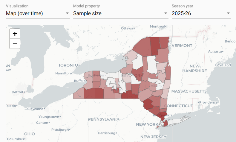
Figure showing simulated mock results for demonstration purposes only.

Visualization type: Time series

Models that produce this output: Models 2 and 3

Model properties: Sample size; Probability of any disease presence; Probability of prevalence ≥ 1.0%

Season-year: Default is the target sample-year, e.g. the upcoming season-year. Users can choose a season-year up to 20 years from the drop-down menu to change the visualization. Any historical sampling data that was used is available only under the sample size model property.

Description:

The top part displays a line graph with a line corresponding to each sub-administrative unit in the model. The time in season-years is given on the x-axis, and the y-axis has the values corresponding to the chosen model property (probabilities are given as the percent value). The grey dashed vertical line corresponds to the selected season-year. The light grey vertical line delineates the historical years of sampling data. Users can hover over the data points to see the area name, year, and corresponding value. Note the change in y-axes scale between the selected model property values.
The bottom part of the page is a table where the rows are the sub-administrative unit, and the corresponding management unit if applicable. The columns are the values at every season-year for 20 years. The bold-highlighted column corresponds to the values in the figure that line up with the dashed grey line, i.e. the values of selected model property in the selected season-year. Users can click on a management unit or area, i.e. sub-administrative unit, which will show only the line(s) corresponding to the selected area(s). Historical sampling are also shown in earlier years if available, delineated to the left of the grey bar, only in the visualization with model property “Sample size”.
Note, the values between the “Map (over time)” and “Time series” visualization are the same, however only 1 year can be visualized on the map at a time, while measures can be plotted over all time points simultaneously in the line graph to observe and compare trends. The tables between these two pages should show the exact same values.
This image can be downloaded using the download icon at the top right of the figure. Note that the scale of the downloaded figure will depend on the scale of the figure in the browser at the time of download.

Corresponding output files: sample_size.csv, probability_disease_present.csv, probability_prevalence_1_0.csv

Figure showing simulated mock results for demonstration purposes only.

Visualization type: Cost analysis

Models that produce this output: Model 3

Model properties: None

Season-year: None

Description:

The top part of the page is a bar graph with a bar for each budget tested, which range from 50-400% of the specified budget (in 10% increments up to 200% and then 50% increments). The height of the bar is the total amount of time (in years) that CWD is expected to go undetected until the first detection (see additional details about this measure under total_unobserved_spread.csv output description). The darker shaded bar corresponds to the user-specified budget.
The bottom part of the page is a table with one row for each budget that was used for calculating an optimal control plan, the corresponding percentage of that budget relative to the user-specified budget, the total amount of time (in years) that CWD is expected to go undetected until the first detection (i.e. the height of the bars), and the relative change in the total unobserved spread compared to the plan on the current budget (see additional details about these measures under total_unobserved_spread.csv output description). The color tags on the left side of the row correspond to the color of the bar.
This image can be downloaded using the download icon at the top right of the figure. Note that the scale of the downloaded figure will depend on the scale of the figure in the browser at the time of download.

Corresponding output files: cost_analysis.csv

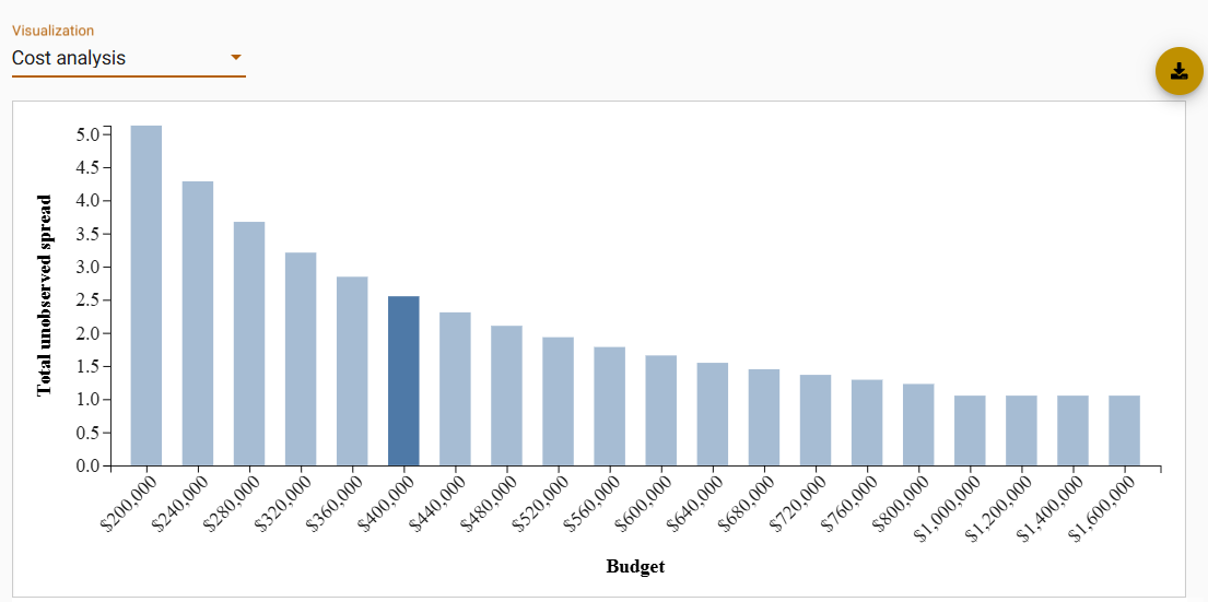
Figure showing simulated mock results for demonstration purposes only.

18.6 Details on the Theory

The theory of surveillance optimization is presented and proved in the manuscript below. Note that this reference details a surveillance strategy and a prevention strategy however the implementation in the warehouse only produces the optimal surveillance strategy at this time.

[1] Wang J, Hanley B, Thompson N, Gong Y, Walsh D, Gonzalez-Crespo C, Huang Y, Booth J, Caudell J, Miller L, Schuler K. 2025. Strategic planning of prevention and surveillance for emerging diseases and invasive species. PNAS. DOI: https://doi.org/10.1073/pnas.2507202122

18.7 Code

The code is publicly available at https://github.com/Cornell-Wildlife-Health-Lab/sample-allocation-model.