Ryan's ECE 4960 Site
Lab 3: Sensors
This lab was dedicated to setting up, installing, and testing the sensors that will be used to give the robot input. These involved two Time of Flight (ToF) Sensors (the VL53L1X) that can be used to measure distances from objects. It also involved one Inertial Measurement Unit (IMU) Sensor (the ICM-20948) that can be used to measure rotations, like pitch, roll, and yaw.
Wiring
Before I began installing and testing the sensors, I first had to plan out where the sensors
should go on the robot and had to figure out the wiring based on these decisions since these
would be soldered connections that would be difficult to undo.
I decided I would put one ToF sensor on the front and one ToF sensor on the side.
Since I assume the robot would mostly be moving forward and turning, this seemed like the optimal
configuration to get the best relevant coverage. I also decided the IMU should be placed somewhere
on the inside of the robot facing directly upwards to make rotation measurements easier.
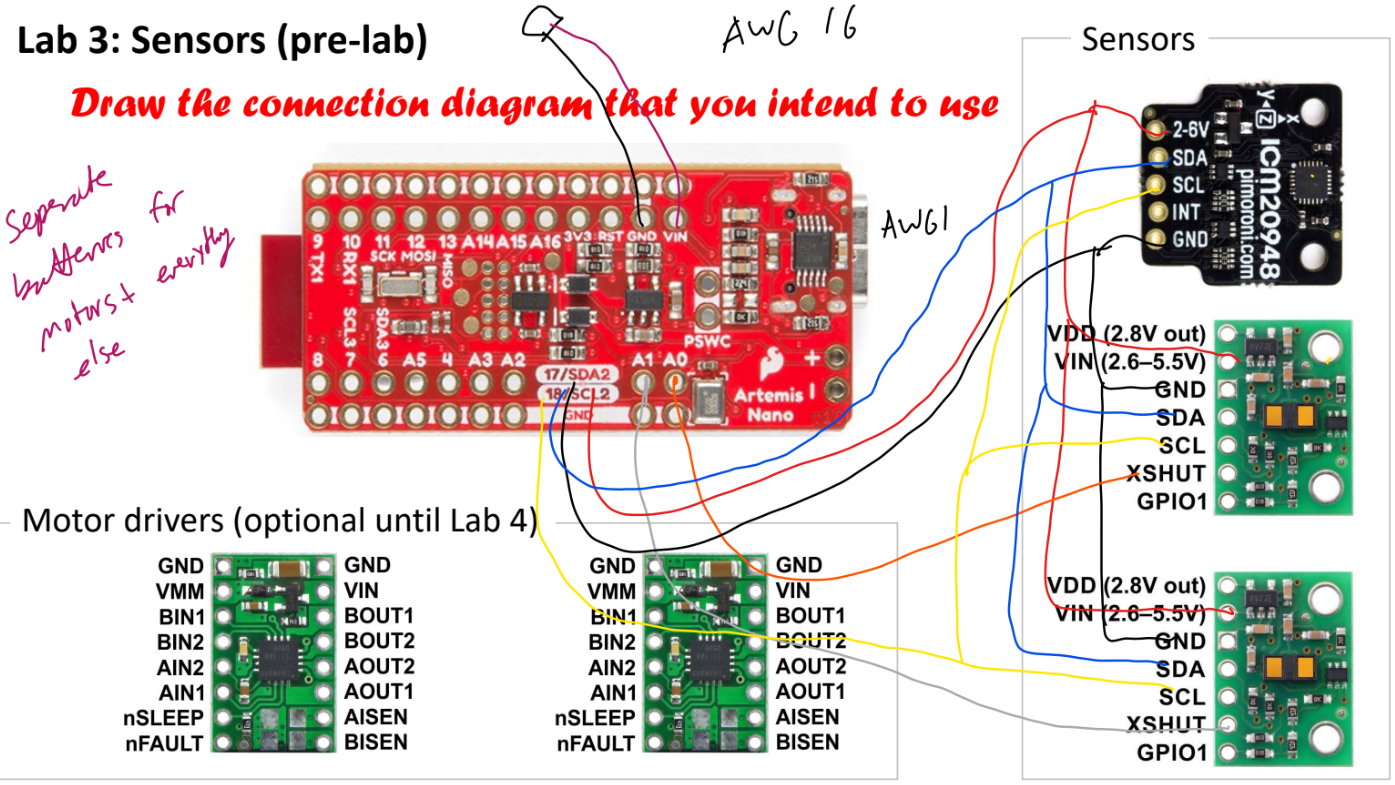
I then worked on planning the wiring, which was mostly just connecting the I2C pins and power pins
to each of the sensors. I drew
these connections on my tablet to plan this out. Once this was
figured out, I cut appropriately sized wires based on the sensor placement described above and
soldered them together.

Time of Flight (ToF) Sensors
I first started with the VL53L1X ToF sensors and wired them based on the diagram I drew above. I then
ran the Wire_I2C example sketch to make sure it was working properly. This outputted an address of 0x29,
which did not match the default address of 0x52 in the VL53L1X datasheet. However, this makes
sense because the address transmission of the I2C protocol has one of the bits as a read/write bit
with the next 7 bits as the address. So if you shift the address one bit you end up
getting 0x52, which is expected.
The VL53L1X sensors have three modes according to the datasheet:
a short distance mode that is the most immune to ambient light
but only has a rated range of ~1.3m, a long range mode that has a much
longer rated range of ~4m but is the most impacted by ambient light, and
a medium distance mode that is somewhere in between in terms of range and
susceptability to ambient light. I chose the short range mode because
I feel that accurate ranging is one of the most important aspects to a
fast robot since it is very reliant on good mapping to function well.
However, the rated range of ~1.3m is fairly short, so this might change
in the future.
I then tested the sensors using the Example1_ReadDistance example sketch with it set to short distance mode. I first tested
the range of the sensors by slowly moving the sensor away from a wall until the data started
to becoming strange (showing distances of 0). I found that the max range of the sensors
is about 2250mm, which is farther than the rated range at short distance, but this was
also tested at night in a farily dark dorm room.
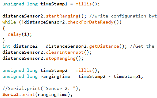
I then tested the ranging time by setting time stamps before and after the measurement and got
and average time of 53ms at 400mm.
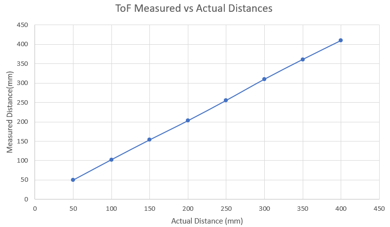
I then tested the accuracy and repeatability by recording and averaging 28 measurements at distances of 50mm, 100mm, 150mm, 200mm, 250mm, 300mm, 350mm, and 400mm. I found that the accuracy was very good for the first ~200mm and then started to diverge slightly after that. I found the repeatability was extremely good with an average standard deviation of 1.07.
| Measurement | 50 mm | 100 mm | 150 mm | 200 mm | 250 mm | 300 mm | 350 mm | 400 mm |
|---|---|---|---|---|---|---|---|---|
| Average | 49.89 | 102.4 | 153.6 | 202.9 | 255.3 | 310 | 360.9 | 409.8 |
| St. Dev. | 1.012 | 0.9056 | 1.342 | 1.209 | 1.042 | 1.133 | 0.9813 | 0.9656 |
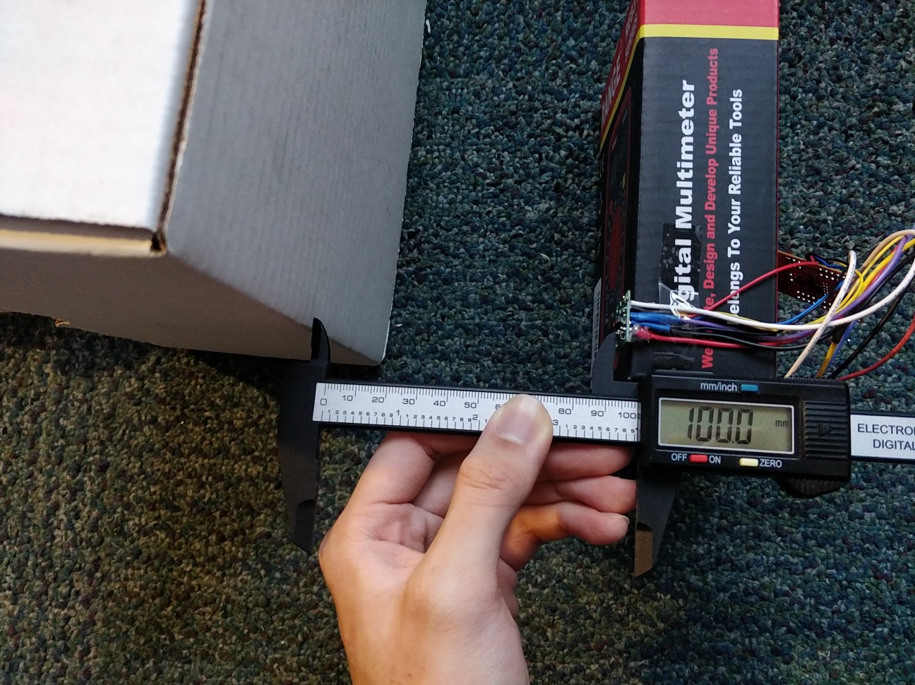
I then repeated the above experiment on a red shirt to see if the sensor is sensitive to different textures and colors. I found the results to be similar to the white cardboard test above.
| Measurement | 50 mm | 100 mm | 150 mm | 200 mm | 250 mm | 300 mm | 350 mm | 400 mm |
|---|---|---|---|---|---|---|---|---|
| Average | 47.32 | 101.4 | 153.9 | 211.2 | 261 | 304.9 | 358.4 | 409.6 |
| St. Dev. | 1.071 | 1.237 | 0.8175 | 1.354 | 0.8864 | 1.187 | 1.608 | 1.144 |


I then worked on getting both sensors working together. Since the ToF sensors had the same address,
my original plan was to solder connections to each
of the ToF XShut pins to turn on the sensor I wanted to use while turning off the other. However,
I found that this required me to reinitialize the sensors each time I wanted to use them, which was
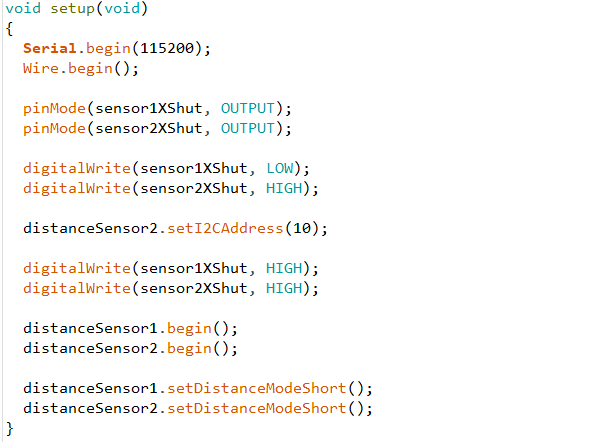
very slow. So I then decided to turn off one of the sensors during setup and set the I2C address
of the turned on sensor to another address so I can avoid the address conflict. This was successful
and I got a significantly higher sample rate.

Inertial Measurement Unit (IMU)
Next, I tested the ICM-20948 IMU and wired them based on the diagram I drew above. I then
ran the Example1_Basics example sketch to make sure it was working properly. In this file,
I had to change the AD0_VAL value, which represents the last bit of the I2C address from 1 to 0.
This is because the ADR jumper is closed.
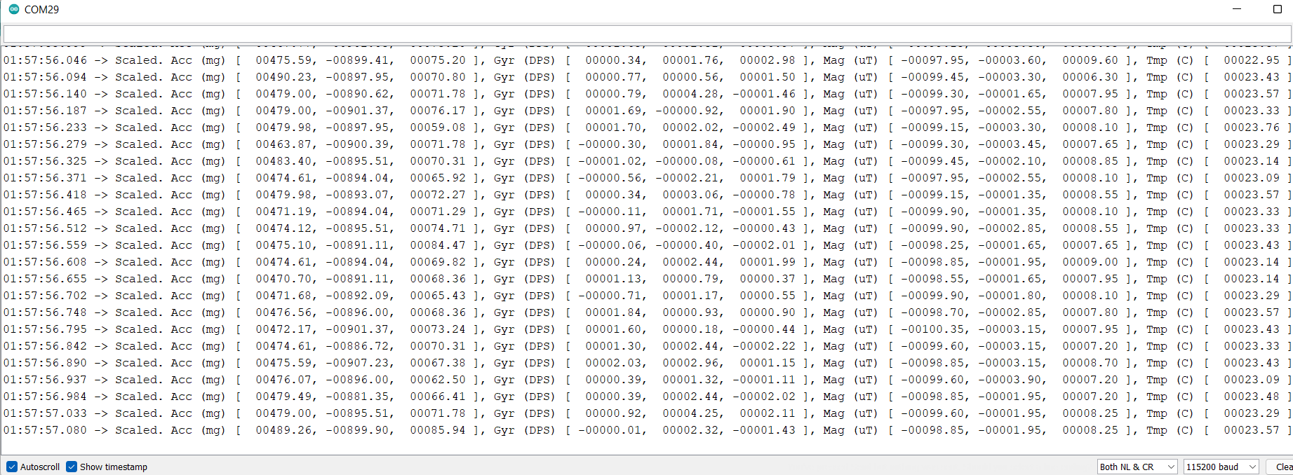
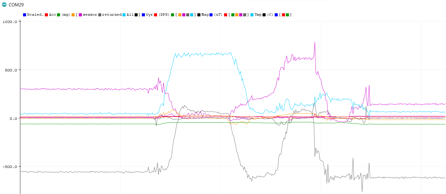
When I opened the serial monitor, I saw the acceleration and gyroscope data for each of the 3 axes.
As I rotated the board the gyroscope data changed, which makes sense since it measures change in rotation
in degrees per second, and I also saw the acceleration change, which also makes sense since it measures the
Earth's gravitational acceleration. When I accelerated the board linearly, I also saw the acceleration change as expected.
Accelerometer
After doing these basic tests, I then wrote code based on the equations from class to convert the accelerometer data into pitch and roll in degrees.


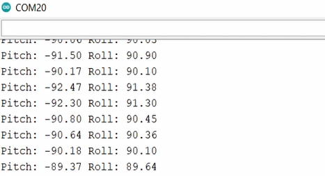
As a test, I rotated the IMU to -90 degrees pitch and 90 degrees roll. I found that this was fairly accurate, being about 4 degrees off when I compared its output to a protractor.
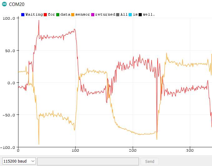
I then plotted the data, which was very consistent with my movements. The red is pitch and the yellow is roll.
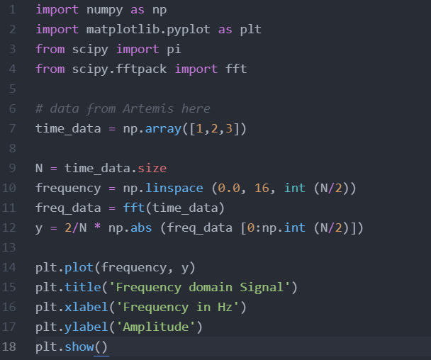
After this, I tried tapping the IMU and plotting the frequency response. To do this, I wrote a Python script to plot the FFT with help from the article provided in the lab page. I then recorded data from me tapping the IMU a few times, and put that data into the time_data variable in the Python script.
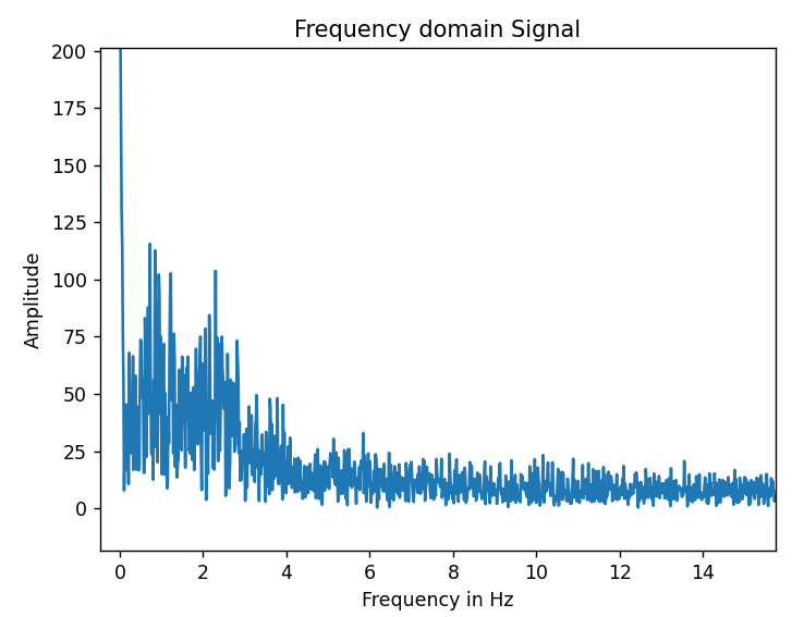
This produced this FFT graph, with a huge spike at around 0 Hz. After zooming in, I see many spikes in the 0-4 Hz range which are likely from my taps. It then starts tapering off, which is likely where most of the unwanted noise lies. From this, I believe that a complementary low pass filter cutoff frequency of about 4 or 5 Hz should work well. This filter should affect the output by attenuating frequencies above the cutoff frequency.

Gyroscope
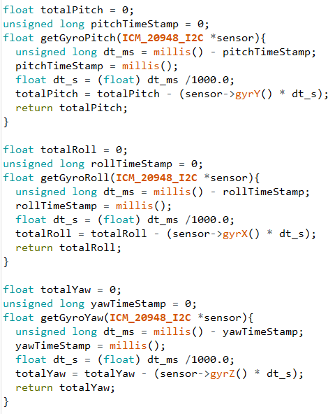
After this, I wrote code based on the equation from class to convert the gyroscope data into pitch, yaw, and roll in degrees.

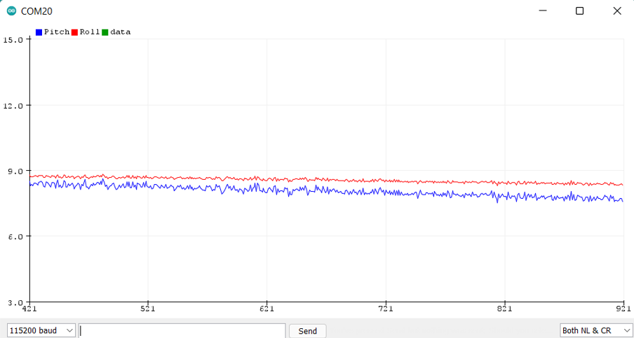
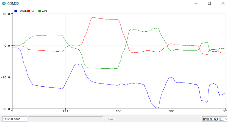
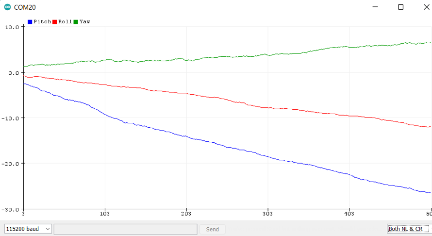
After plotting the data (left), I noticed that the output values were significantly smoother compared to the values from the accelerometer. However, it did drift, which did not occur with the accelerometer. This drift can be seen clearly in the plot on the right, where I am not moving the IMU at all
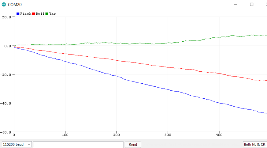
I tried lowering the sampling frequency by increasing the delay in the loop from 30ms to 60ms, but this didn't seem to affect the drift or accuracy much.
Complementary Filter
Finally, I implemented a complementary filter that combined the gyroscope and accelerometer data. It had an alpha value of 0.5 that I found gave me very good results. Combining these two input methods produced data that had the best of both words: the accuracy and lack of drift from the accelerometer and the low noise of the gyroscope. Below is a video demonstrating it in action. Below is also an image showing its lack of drift.
