Ryan's ECE 4960 Site

This lab was dedicated to implementing a Kalman filter, which should help make it easier to accomplish the PID task from the last lab faster.

Step Response

A Kalman Filter requires an A, B, and C matrix to work. From lecture, we derived these state space equations for Task A:

Therefore, with the above equation, I just had to find d and m to complete the A and B matrices. To do this, I first drove the robot forward towards a wall while logging motor and ToF data as it reached a steady state constant speed. Graphs of the data are shown below (note that I added in a sharp reverse at around 300 mm to prevent damage to the robot from ramming into the wall. This explains the somewhat strange values at around the 77 second mark):

Reaching steady state (constant) speed is important, because it lets me use this equation from lecture to calculate d:

From my data, I found the steady state speed to be around 1767 mm/s. Plugging this and u = 1 into the above formula gives me d = 0.00057

Next, I found m by using this formula from class:

The formula requires a 90% rise time which I found to be 1.41 seconds from my data. Plugging this and d = 0.00057 into the above formula gives me m = 0.00035

Now knowing d = 0.00057 and m = 0.00035, we can plug these values into the state space equations above to get our A and B matrices:

Kalman Filter Setup

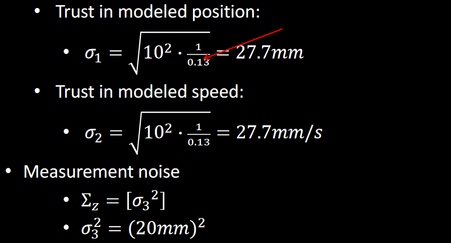
The Kalman filter also needs process noise (Sigma_u) and a measurement noise (Sigma_z) covariance matrices.

To find these values, I decided to come up with ballpark values and will later tune them based on my results. For these ballpark values, I decided to use the values given in lecture:

Sanity Checking the Kalman Filter

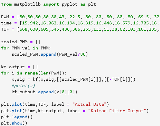
To check that the Kalman Filter works, I first ran it in Jupyter using Python with pre-recorded data from the last lab. This involved combining the A, B, and C matrices as well as the process and measurement noise and covariance matrices found in the previous parts into this code:

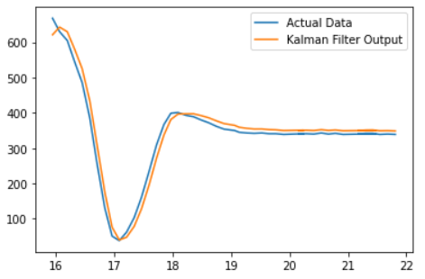
Using the parameters defined in the code above, I plotted the output of the the Kalman Filter function versus time. The output matches the actual data very well:

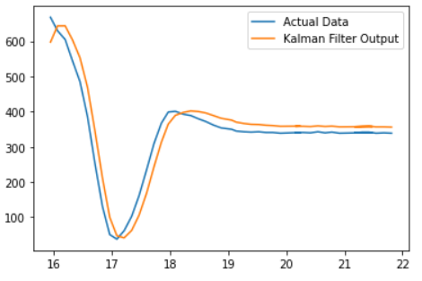
I next reduced the Sigma_z to be 200 instead of 400 which would cause it to trust the sensor more than the model. As expected, this caused the KF output to match the actual data more closely:

Implementing the Kalman Filter on the Robot

After confirming that my Kalman Filter worked on the pre-recorded data in Python, I next implemented the Kalman Filter on the Robot by translating the Python code line-by-line into Arduino C. This was a bit difficult to do since the the Arduino library to work with Linear Algebra was more finicky than NumPy, and C is generally harder to use than Python especially for these types of tasks; I'm glad we sanity checked it in Python first. Here is the Kalman Filter itself in Arduino C, with the matrix definitions on the left and Kalman Filter function on the right:

Using the Kalman Filter in my PID code was very easy; I just swapped the actual data for the Kalman Filter output to calculate the error and everything else stayed the same:

I next tested the Kalman Filter on my robot, and it worked very well:

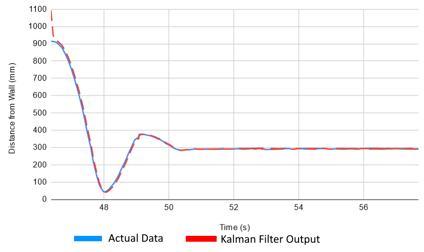
After plotting the recorded data from the robot, I saw this was mostly because its Kalman Filter prediction matched very closely to the actual measurements from the ToF sensor: