Materials

• A Laptop

Computer Setup

To get the simulator up and running, we have to do download and configure a couple packages on our system. Since I have a Mac laptop, I did the following steps.

                    $ python3 --version
                    $ python3 -m pip --version
                    

Install all the Python dependencies and setup the virtual environment as we did previously in Lab 2

Install pip Packages

                          $ python3 -m pip install numpy pygame pyqt5 pyqtgraph pyyaml ipywidgets colorama
                    

Install Box2D Package

                        
                    
                    $ source ece4960_ble/bin/activate
                    # Download pip wheels

                    $ pip install --find-links <wheel_directory> box2d
                    $ python
                    >> import Box2D
                    >> print(Box2D.__version__)
                    2.3.10
                    

Simulator Setup

1. Download and extract the simulation base code into the project folder
2. Downaload the Lab 10 Notebook and copy lab10.ipynb into the notebooks directory (inside the simulation base code directory)
3. Follow the instructions in the notebook to understand how to control your virtual robot and use the plotter

Lab Taks

Simulator Functionalities

You can start, stop, and reset the simulator and plotter with the following functions:

• Simulator:
  1. START_SIM()
  2. STOP_SIM()
  3. RESET_SIM()
• Plotter:
  1. START_PLOTTER()
  2. STOP_PLOTTER()
  3. RESET_PLOTTER()

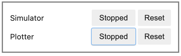
Alterntively, we could use the GUI interface as shown below to toggle the start, stop, and reset buttons for the simulator and plotter

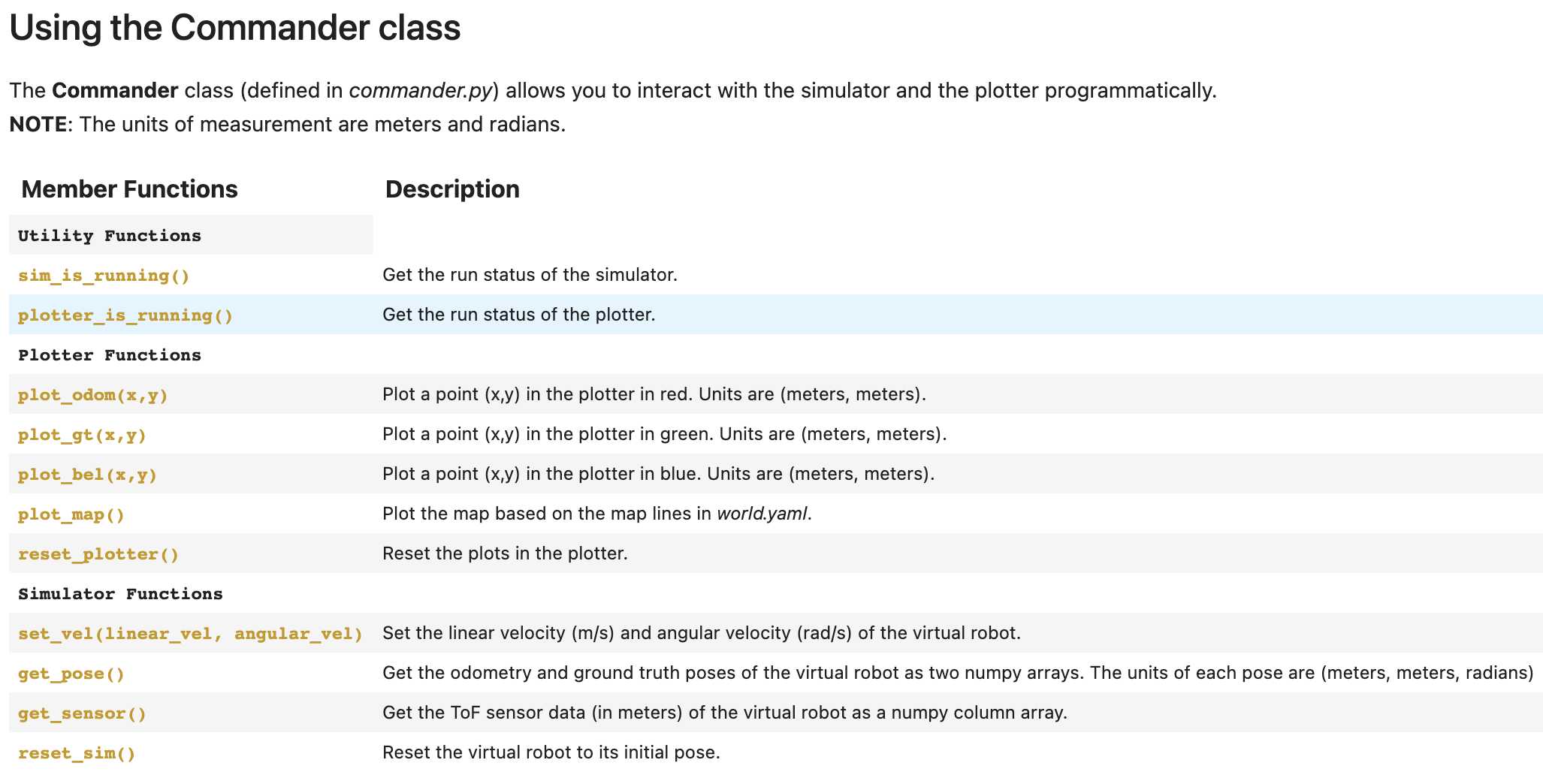
Shown below are all the member functions of the comander class, which allows you to interact with the simulator and the plotter programmatically.

Simulator User Input

There are a few other ways to interact with the virtual robot. You can either use a mouse or a keyboard. To interact with the simulator you can do the following.

• Press the up keys to increase the linear velocity of the virtual robot.
• Press the down arrow keys to decrease the linear velocity of the virtual robot
• Press the left arrow keys decrease the angular velocity of the virtual robot.
• Press the right arrow keys to to increase the angular velocity of the virtual robot
• To stop the robot press the spacebar key
• Hit the "H" key to display the full keyboard map.

Open Loop Control

In this lab segment, we were tasked to perform a “square” loop in the map. To do this I leveraged the commander class member function set_vel() to define the linear and angular velocity. The inputs into the set_vel function were found via trial and error. Next, I inputed a constant time for the virtual robot to drive forward and turn. Below you can see the program I used to execute this along with the demo video of the virtual robot performing the square loop.

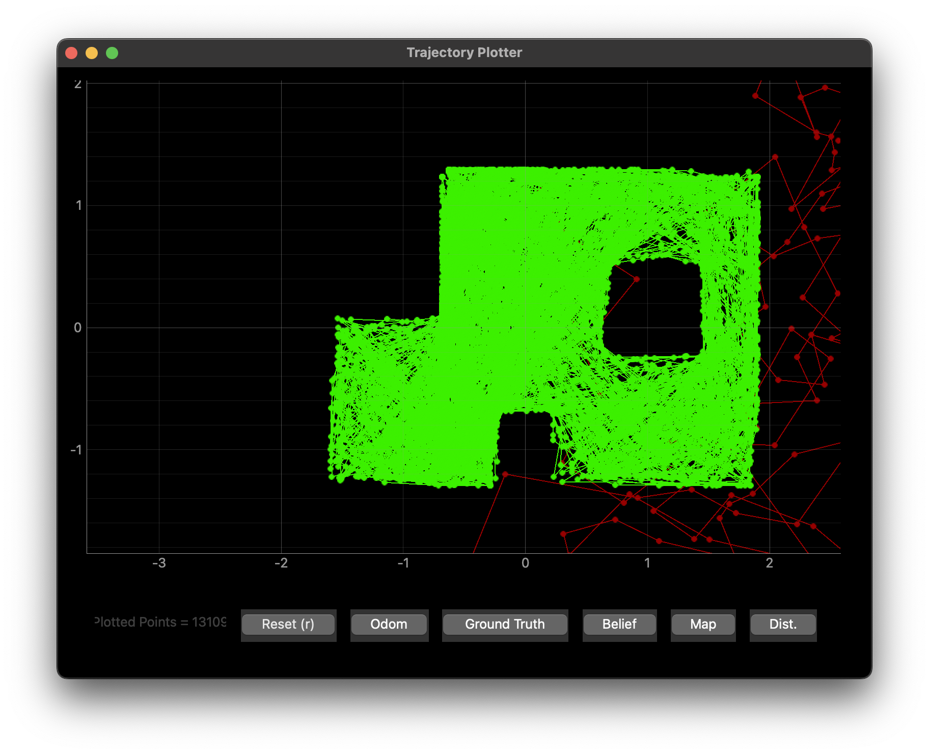
The plotter displays two plots (One in green and Red). The green plot shows the actual path of the simulated robot a.k.a ground truth, while the red plot is the odometry data, which is just the robot sensor information. In theory the odometry and gorund truth readings should be the same, but because the odometry data accounts for noise and the IMU sensor data is simulated as well, the resulting effect is an odometry and ground truth plots with heavy disparities.

Closed Loop Control

Next we design a simple controller in python to perform a closed-loop obstacle avoidance.

By how much should the virtual robot turn when it is close to an obstacle?

Based on trial and error I realized that the best value for turning was ~ 1.56 rads/s which is about 90 degrees. With a 90 degree turn, the virtual robot is able to do incremental but non-exhaustive scan of its environment to find an obstacle free path.

At what linear speed should the virtual robot move to minimize/prevent collisions? Can you make it go faster?

Using velocity of 0.5m/s, the robot was able to navigate very well with minimal to collisisons. However, as the velocity was ramped up to 3m/s, the frequency of collision increased and there was an even more drastic difference at 4m/s. Consequently, I would conclude that a velocity of 3m/s or less is good range to use to keep the virtual robot free of collisions and obstacles along its path.

How close can the virtual robot get to an obstacle without colliding?

From the experiments, I ran with my robot at a speed of 0.5m/s, I realized that 0.5m was the threshold distance that the robot can handle before collisions. As a result, I would summise that a distance of 0.5 meters and below is more a less a good threshold distance for avoid obstacles.

Does your obstacle avoidance code always work? If not, what can you do to minimize crashes or (may be) prevent them completely?

The obstacle avoidance doesn't always work and this is very evident whenever the robot comes in at a slight angle. I reckon this is probably due to the fact the Field of View of the robot is very limit and thus does not account for situations where the corner of the car collides with the wall. This problem could perhaps be solved by adding two ToF sensors on the sides to compensate for the front ToF lack of vision in its blindspots.

SOMETHING COOL

So I accidently left obstacle avoidance program running for a couple of hours and plotter essentially plotted out the density function of the robot's position over time. I suppose this could be used to persuade the teaching staff that my obstacle avoidance program runs well, as the areas without plots clearly define the boundary / confines which the robot cannot go to and through.