Lab 11: Localization (Simulation)
Objectives:
The main objective of this lab is to implement grid localization using Bayes Filter.
Materials
- A Laptop
Lab Taks
Grid Localization
The robot state is 3 dimensional and is given by the
parameters .
The robot’s world is a continuous one that is confined
by the following boundaries:
- [-1.6764, +1.9812) meters or [-5.5, 6.5) feet in the x direction,
- [-1.3716, +1.3716) meters or [-4.5, +4.5) feet in the y direction,
- [-180, +180) degrees.
However, to work with these values in the simulation, they are instead discretized by cells. Ultimately this allows us to compute our beliefs over a finite set of states in a resonable amount of time. With tis modification we now have the following boundaries to work with.
- [0,12) for x cell,
- [0,9) for the y cell
- [0,18) degrees per cell
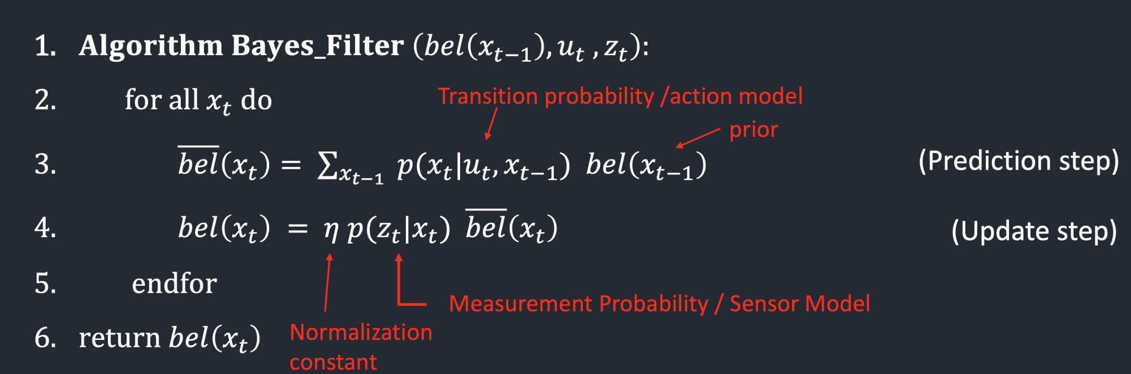
Bayes Filter Explained
To complete this task of localization, we leverage the Bayes Filter algorithm shown in the figure above and implement it in python. In the simplest way possible, the Bayes algorithm takes an initial probability that we have of the robot being in a certain position/state, and then iteratively updates the belief using the control input we feed in to the system and the sensor measurements that it receives. This algorithm is very robust to noise, so with the many iterations of the conditional probabilities that it calculates, the predicted state is very close to the ground truth measurements.
Algorithm Decomposed
There are three inputs into the Bayesian Filter:
- bel(previous_state) → This is the prior (previous belief) of the robot. In the python implementation this represented by a 3D matrix of probabilites associated with the robot being in each state
- u → This is the control input that we fed the robot to move from its previous position to its current one . In the implementation, it has parameters delta_rot1, delta_rot2, and delta_trans.
- z → This is the real time sensor measurements of the robot. It's represented by 18 data points that the robot retrieves every 20 degrees as it spins 360 degrees.
Iteration
- Xt → During the iteration Xt, all possible
current states of the robots are checked. In our
discrete model, we check for the entire set of
possible
values that the robot may take
Future Predictions
- bel_bar(current_state) → This refers to the variable responsible for holding updated versions of the robot's prior belief.
- p(current_state | u, previous_state) → This quantifies the chance (probabilites) that you robot is in the current_state given that it received a particular control input (u) and it was at a previous posiiton denoted by previous_state.
- bel(previous_state→ This is the same definition as the one in the above input section
These variables are the summed up over all possible prior states that robot could have possibly been in.
Updating the Belief
- bel(current_state) → This represents the belief that robot is in the current state. Note that bel(previous_state) will take this value in the next round of iteration
- η →This serves as a normalization constant. This is necessary for our belief / probabilites to add up to 1
- p(z | current_state) → refers to the probability that given the current_state of the robot, the 18 measured sensor readings for the 360 scan are correct.
- bel_bar(current_state) → has the same definition as the one in the prediction step
Bayes Filter Implemented
Compute Control
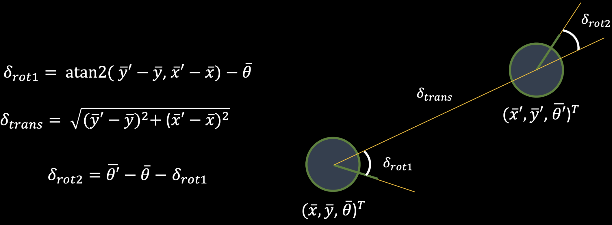
Compute control is a function that generates a control input (u) given data of a current and previous state of the system. In particular, it yields three values of values of interest — 𝜹_rot1, 𝜹_rot2, and 𝜹_trans.
- 𝜹_rot1: The rotational change from the starting angle
- 𝜹_rot2: The rotational change from the ending angle
- 𝜹_trans: The Euclidean distance between the starting and ending points
Odometry Model
The odometry motion model is responsible for computing the probability that robot ends up in a current state given a previous state and a control input. The odometry function has three parameters for computation:
- Control input (u)
- Current_state(Xt)
- previous_state(previous_state)
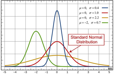
Anyways to generate the probability of interest, as mentioned above, we rely on a Gaussian distribution. This distribution function requires a 𝝈 value which indicates the variance of values relative to its expected value (μ) which is another parameter it has and an input X, for which we want to solve the probability of realizing. For reference, I've attached a figure of Normal distribution with μ = 0 and 𝝈 = 1. First we need to extract the probabilities of 𝜹_rot1, 𝜹_trans, and 𝜹_rot2 repectively using the guassian function and then multiply them together to attain the probability of that robot ends up in a current state given a previous state and a control input. Important to note is that we are given a particular 𝝈 values for 𝜹_rot1, 𝜹_trans, and 𝜹_rot2 to use for the gaussian function, so we didn't have to derive the variance from scratch.
Sensor Model
The sensor model calculates the probability that the sensor reading from the robot is correct, conditioned on the current_state of the robot. Much like in the last section, we also use the gaussian function for computing the probability (𝝈 is also given to us for this Model).
This model has one parameter:
- Obs which is an array of size 18 featuring the measurements retrieved an arbitrary x,y,θ position in the robot world. In the gaussian function used for computing this probability, these values serve as the μ argument.
The other missing argument for the gaussian function in this section is loc.obs_range_data which represents the current measurements read while the robot scans 360degrees. Since Obs is a size 18 array I iterate through each value when calculating the gaussian and appennd the probability to an array
Prediction
The prediction step leverages the current and previous state given by the sensors of the robot. It uses this information to compute a control input (u) which serves as prior for the prediction step. In this step, we use a total of 6 nested loops to step through every possible previous state (x,y.a) for each current state that we could be in [curr_x, curr_y, curr_a]. This is because every state in "bel_bar" needs to be updated based on "bel" from the previous time step and the odometry motion model.
Nonetheless,executing six loops in this function is quite computationally demanding thus I only iterated through cells if it had a belief probability higher than 10e-4 otherwise I would waste time calculating cells that practically had probability of zero. LAstly I normalized the loc.bel_bar variable to make sure that total probability would sum up to 1 as required.
Update
To update the beliefs of the Bayes Filter, we loop through all possible curent states of the robot by iterating through all values within our discrete [x,y,θ] world. We find our trasitional probability loc.bel_bar for each possibility and multiply it by the conditional probability that our sensor measurement at the robot's immediate state is accurate given that we are at that current state. The belief is then updated for each iteration and then normalized at the very end so that the probability distribution can add up 1.
Results (Videos)
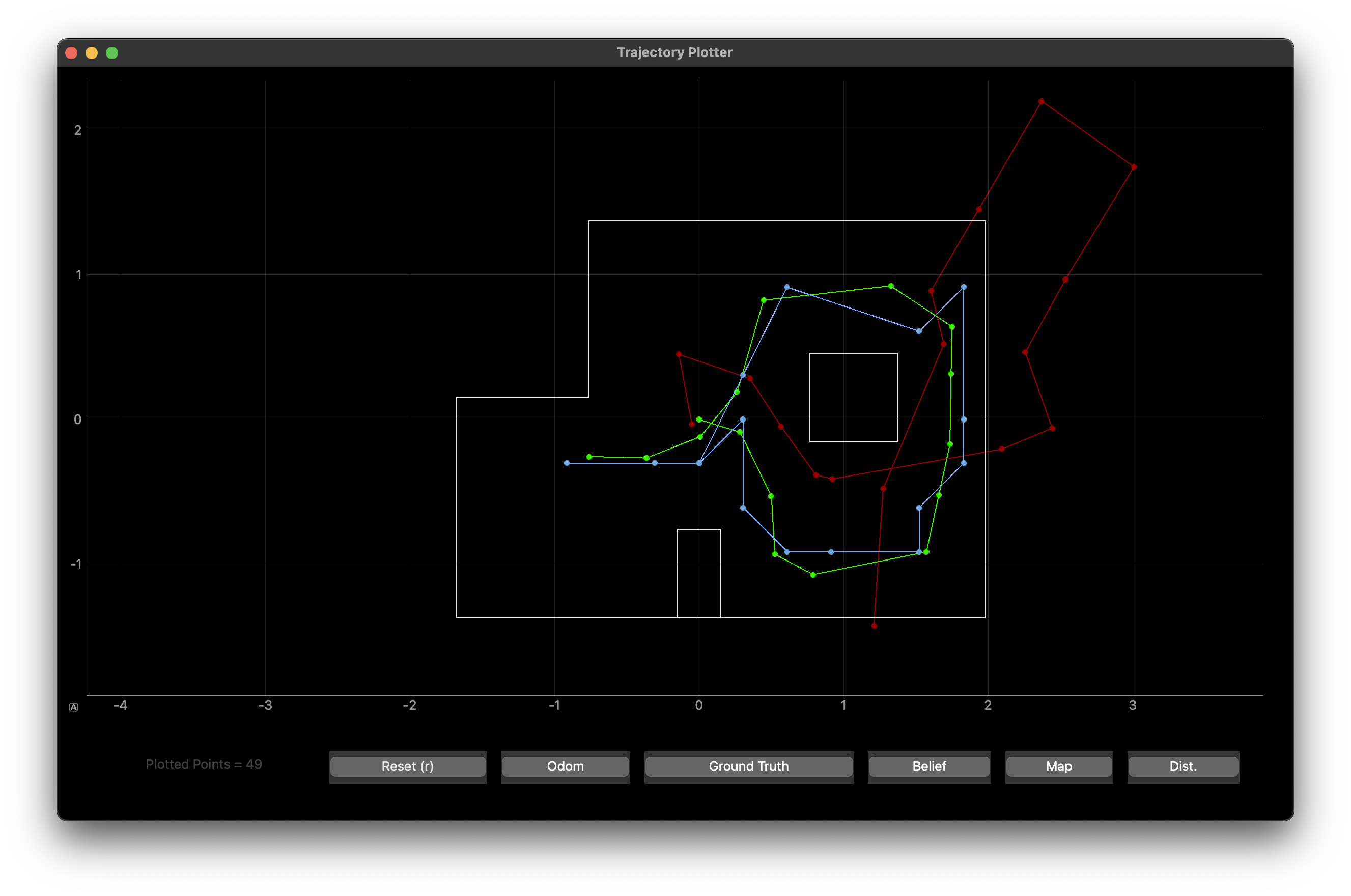
Plotting the odometry (red), ground truth (green) and belief (blue)
- Odometry: Red
- Belief: Blue
- Green: Ground Truth
Plotting the odometry (red), ground truth (green), belief (blue) and the marginal distribution bel_bar(x,y) in the 2d grid space.
>Path Execution
This was the path summary my robot executed given the implementation of the Bayes filter.