Lab 7: Kalman Filter
Objectives:
The objective of this lab is to implement a Kalman Filter, which will help to compensate for the slow sampling rate of the sensors and eventually help execute the PID behavior from Lab 6 much faster, such that stunts can be achieved in future Labs.
Materials
- 1 x Fully assembled robot, with Artemis, batteries, TOF sensor, and IMU.
Lab Tasks
Step Response

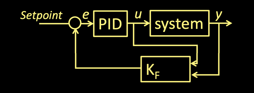
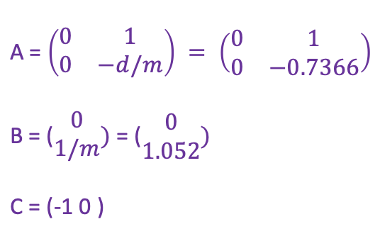
To compute the Kalman Filter we requires three matrices A, B, & C of the form displayed in the above figure. In this lab we assume the scalar u to be 1 and the C matrix to be the same as shown in the figure, thus we only need to solve for the A and B matrices. To find the values of these matrices, we firsty apply a step response to the robot car. In particular, we are looking the effective drag (d) and mass (m) values associated with our system.
Drag
To find the drag value, I applied a step response with a PWM value of 70 for about 4 seconds, just enough to get the car to a steady state velocity. At steady state, the car no longer accelerates but rather coasts at a fixed speed.
When I first applied the step response, I was struggling to realize a steady state speed for the car as the retrieved data would show that the car's velocity plot never had a slope of zero (an indication of steady state) before the end of the step response. See the velocity graph within the figure below to see the behavior I'm referring to.
Starting Point Under 4 Meters
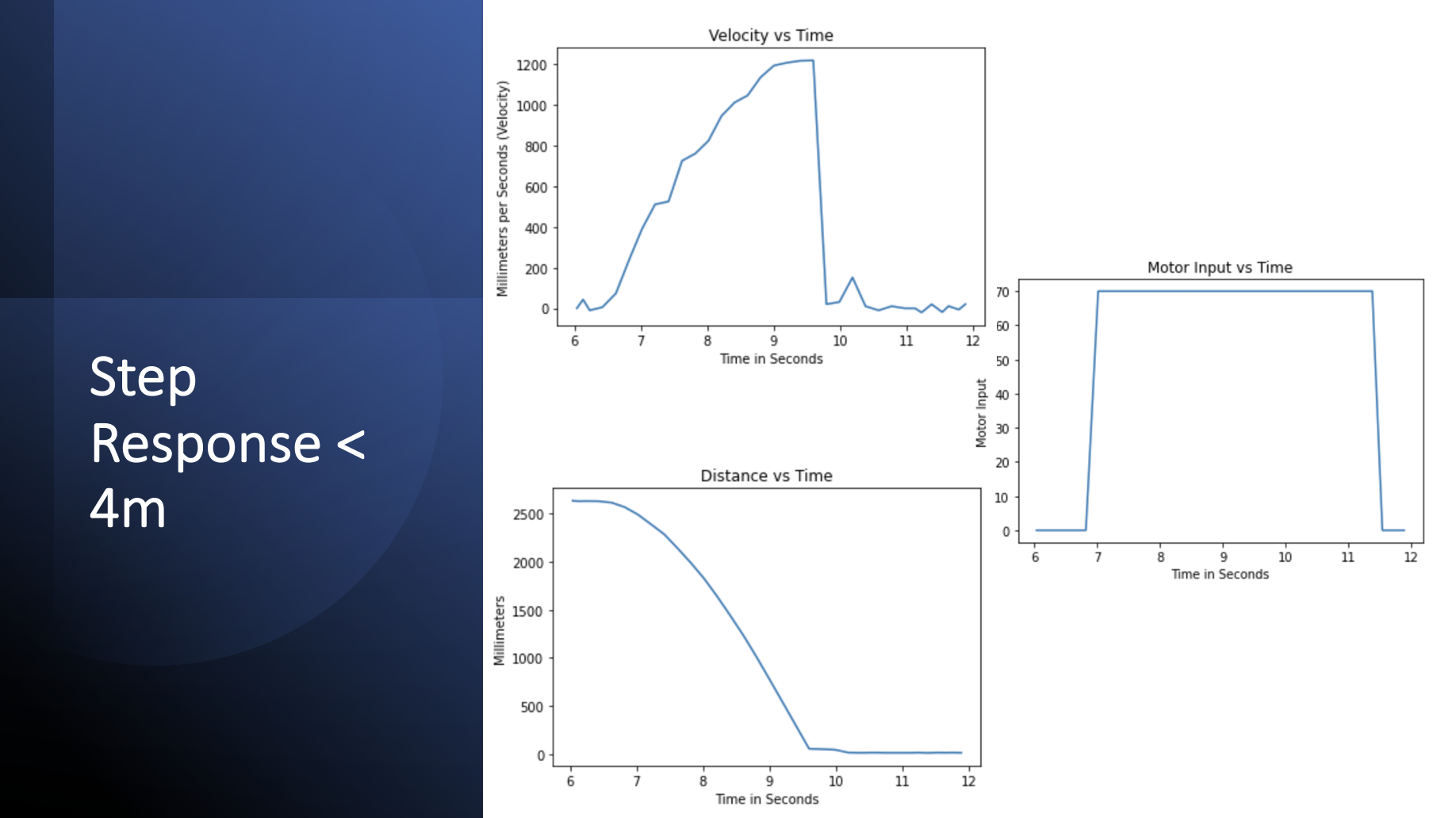
I realized that this issue was a function of the starting distance relative to the end point of the car. I discovered that applying the step response for 4seconds with a starting point under 4meters away from my destination impeded the car from achieving a constant speed but above 4m the car could reach a steady state speed. Observe the plot above to plot below to see the difference in the relative slopes of velocity graphs before the end of the step response/
Starting Point Above 4 Meters

Nonetheless, with the steady state speed achieved, I took the value from the velocity graph and plugged it into the following formula to extract the drag value. You'll notice that in the flat slope region of the velocity plot, the velocity has a bit of noise to it, so to remedy the situation I averaged the peak speed value along with the values just right and left of it and used the result as my input into the formula. The result showed a steady state speed of 1.394m/s. Note here that u equals 1 and Xdot equals the velocity.
Mass
To compute for the mass I needed the 90% rise time of the car. The 90% rise time is the time it takes for the car to reach 90% of the steady state speed I computed above. From the velocity data, I found the rise time value to be 3.05 seconds. Using this value as input into the following formula, I solved for the 'mass' of the system.
With these two values solved for, we have all the neccessary matrices for the Kalman Filter computation.
Kalman Filter
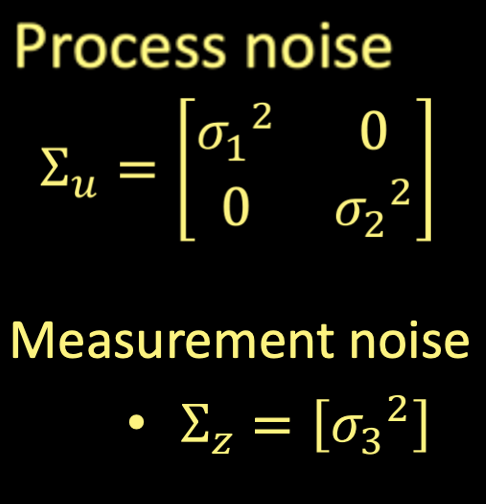
In this segment of the lab, I established the sensor and process noise covariance matrices. The process noise matrix requires two covariance values and the sensor noise matrix only requires one. These covariance matrices essentially quantify how much trust we are currently placing in our model versus the actual measurements we are retrieving from the sensors. Much like in the PID control lab, there's definitely a balance we want to strike and an element of tunning associated with picking the right values for these matrices. In the following section, we explore the effects that different covariance values have on our system. Shown below is the form of these covariance matrices.
Initial Kalman Filter (Sanity) Test
Using the A B C matrices from above along with covariance matrices, I calculated the Kalman Filter estimation. Important to note here is that we discretize the A and B matrices to compute the Kalman model. See the code snippet below for reference.
My analysis of the Kalman Filter is based mostly on the effects of the modification of the covariance matrices. Below I include the results of my starting values followed by the behavior of the model with more sensor noise and also with more model noise.
KF results (Offline)
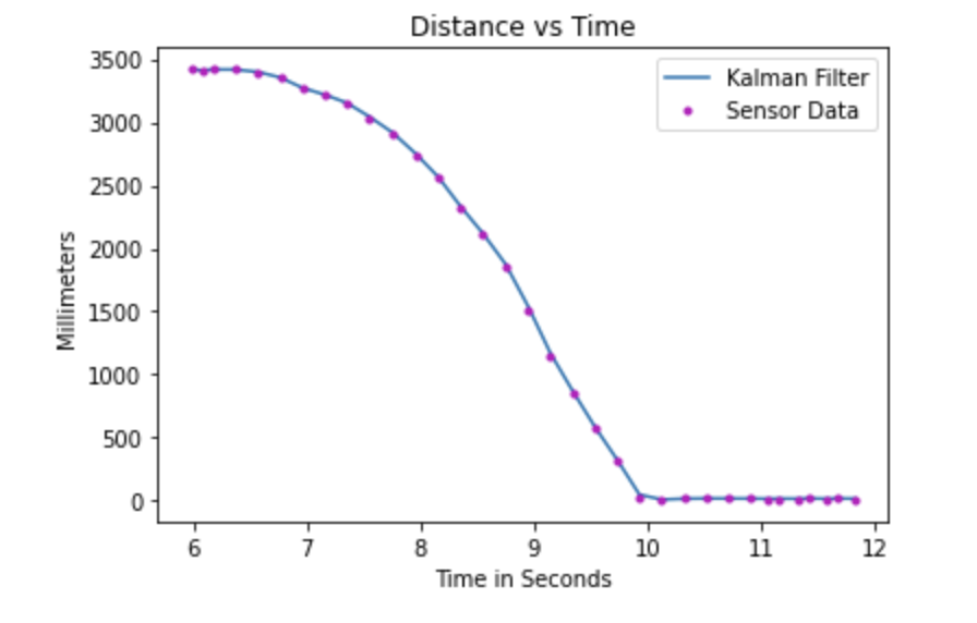
First Attempt: Inital Values / Trust in Model
With an existing data, I had from a previous attempt, we see that putting more trust in the model for this dataset, under compensates for the ability of the system. The model predicts that the car doesn't reach the distance that it actually measured and thus we see the inefficiency of the model when we rely more on it than the sensor.
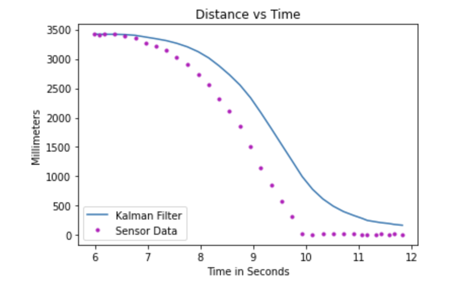
Second Attempt: Trust in Sensor
In this plot, the behavior of the Kalman model fits very closely with the actual data because we placed more emphasis on the sensor readings rather than the predicted values of the filter. This is ideal as the filter works well with the data and doesn't exhibit too much variation.
TOO MUCH trust in Model
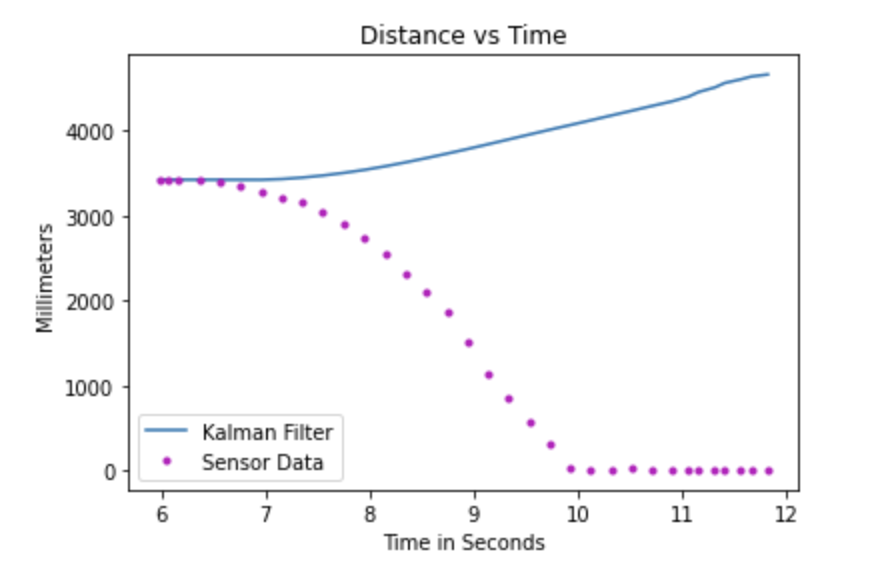
In this plot, I basically place all my trust in the model and it breaks my heart:( ... Just Kidding! The outcome is that the model does break and becomes entirely unrealistic because the data original data suggests an decreasing trend but the Kalman model actually suggests the exact opposite which is not at all what happens.
From these runs, I got a better intuition for the behavior of the Kalman Filter as a whole and went ahead and implemented it on my robot.
Kalman Filter On Robot
In this portion of the lab, I just integrated the Kalman Filter with the PID control loop from last lab and attempted PID control w. the filter. Much like in the previous section, I tested the control sequence with different covariance matrices and below is results they yielded.
KF Results (Online)
Trust in Sensor

I place emphasis on my sensor readings and model follows the sensor readings as expected.
Equal Trust in Sensor With Lower Noise magnitude
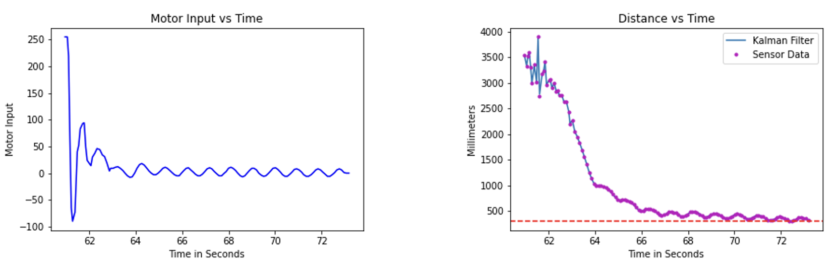
Here the model follows the data extremely well, even though I put equal faith in the model and sensor.
Equal Trust in Sensor With Higer Noise magnitude
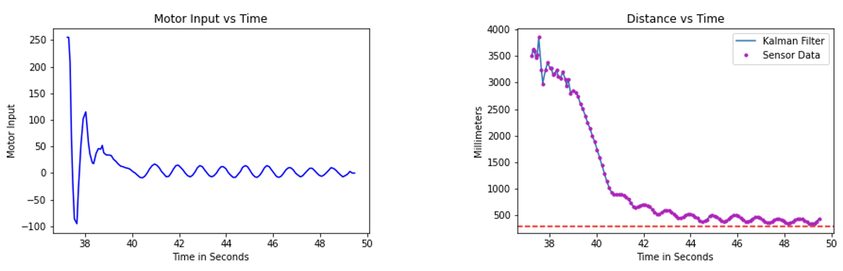
Here, I still put equal faith in the the model and measurement readings and the model still follows the data very well but there's a slight nuance here. Because the noise magnitude is much higer than in the previous equal trust scenario, the model under compensates below the target distance. You'll notice this if you compare the last few data points of this plot against the other similar scenario.
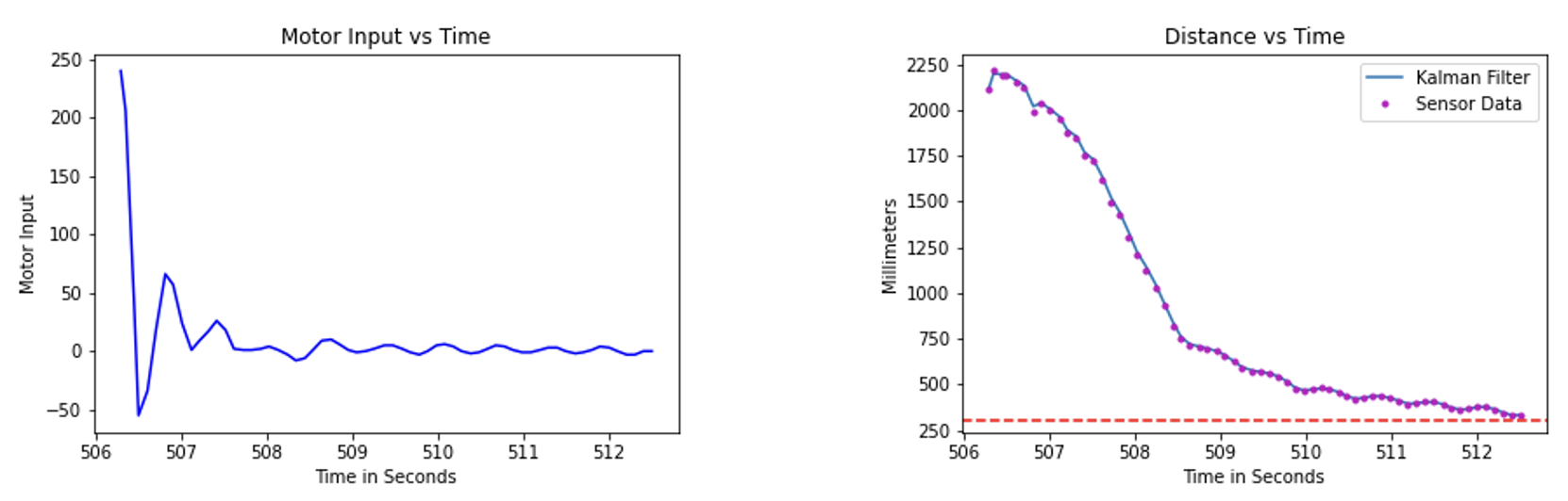
TOO MUCH Trust in Model
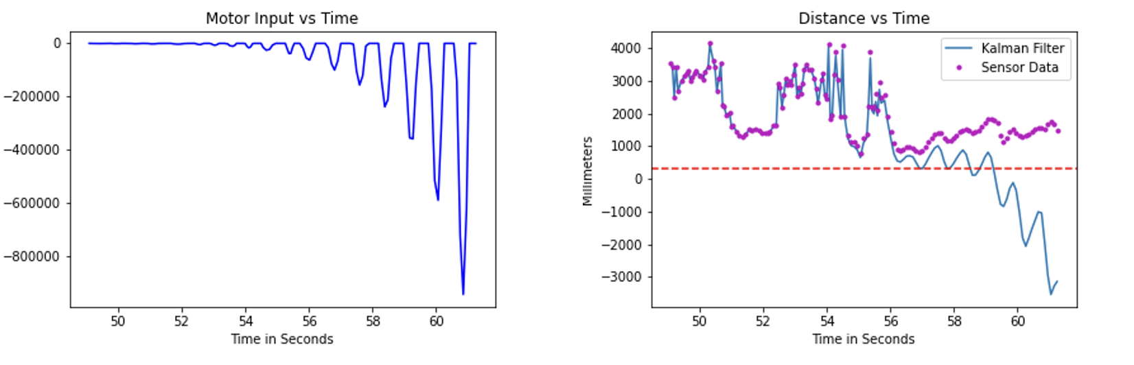
I place too much trust in the model here, and erratic behavior occurs as a result. Worthy of note is that behavior associated with this particular covariance matrix values was awfully similar to the same trend that you'd get out of a derivative kick, if you were solely doing PID control. You can see this by looking at ringinging phenomenon in the motor inputs for these values.
Conclusion
To wrap this lab up I ended up implementing a PD controller to suppress the ringing effects of the P-controller I initally programmed in the previous lab and relied on a covariance matrix with equal trust in both the sesnsor and model. Below is the final result.