Lab 12: Localization (Real)
Objectives:
The main objective of this lab is to perform localization, using only the update step of the Bayes filter, on the physical robot. Let's see how how it goes and maybe we might appreciate the differences between simulations and real-world systems.
Materials
- 1 x Fully assembled robot, with Artemis, TOF sensors, and an IMU.
Lab Taks
Code Verification
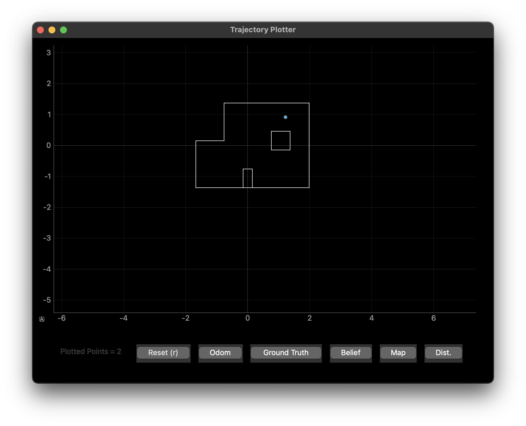
Since we were provided the localization code for this lab, I tested for correct function by running the robot simulation python script and verified for correct behavior. Below is the output of the trajectory mapper using the pre written localization code.
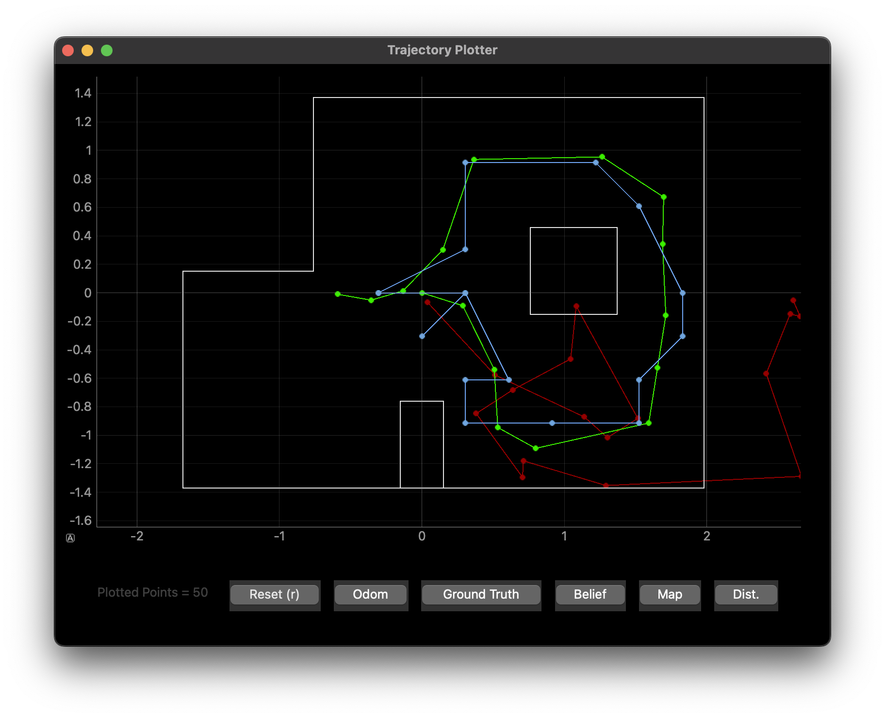
Plot Legend
- Odometry: Red
- Belief: Blue
- Green: Ground Truth
Once I verified that the localization program was functioning as intended, I had to use an observation algorithm in correspondence with the localization code to identify the robot's position in the 4 marked spots in the lab listed below. The marked spots below are all in feet and are relative to (0,0) reference point in the Lab.
- (-3,-2)
- (0,3)
- (5,-3)
- (5,3)
Observation Algorithm on Robot
To complete this task of localization, I leveraged the room scanning program used in Lab 9 to get the ToF sensor readings. However, I had to adjust the code such that I would get 18 sensor readings 20 degrees apart. I attempted to implement a PID controller for the angular speed using the sensor data from the gyroscope, but that was unfruitful as the predicted localization was awfully inaccurate. I think this problem happened because of heavy drift in the gyroscope associated with the rotational speed, ω, of my robot as it was spinning. Nonetheless, I ended up implementing continuous rotation on my robot. More concretely, I had the robot rotate for a sufficient amount of time such that it would able to pick 18 data points from the ToF.
Localization (Real)
In this lab we only use the update step for the localization and this is based the sensor model. As a result, we need only to get the sensor data at a particular point to localize the robot. Thus, in Jupyter Notebook, I only needed to implement one function: perform_observation_loop() which essentially extracted and parsed the ToF data from the Robot's 360 scan and converted into a Numpy Array. Instead of implementing this function from scratch, I integrated a good amount of code from my Lab 9 Jupyter notebook to aid with the extraction of the Robot ToF data. This such a timesaver as it allow for my code to be modular and thus my perform_observation_loop() function only three lines of code.
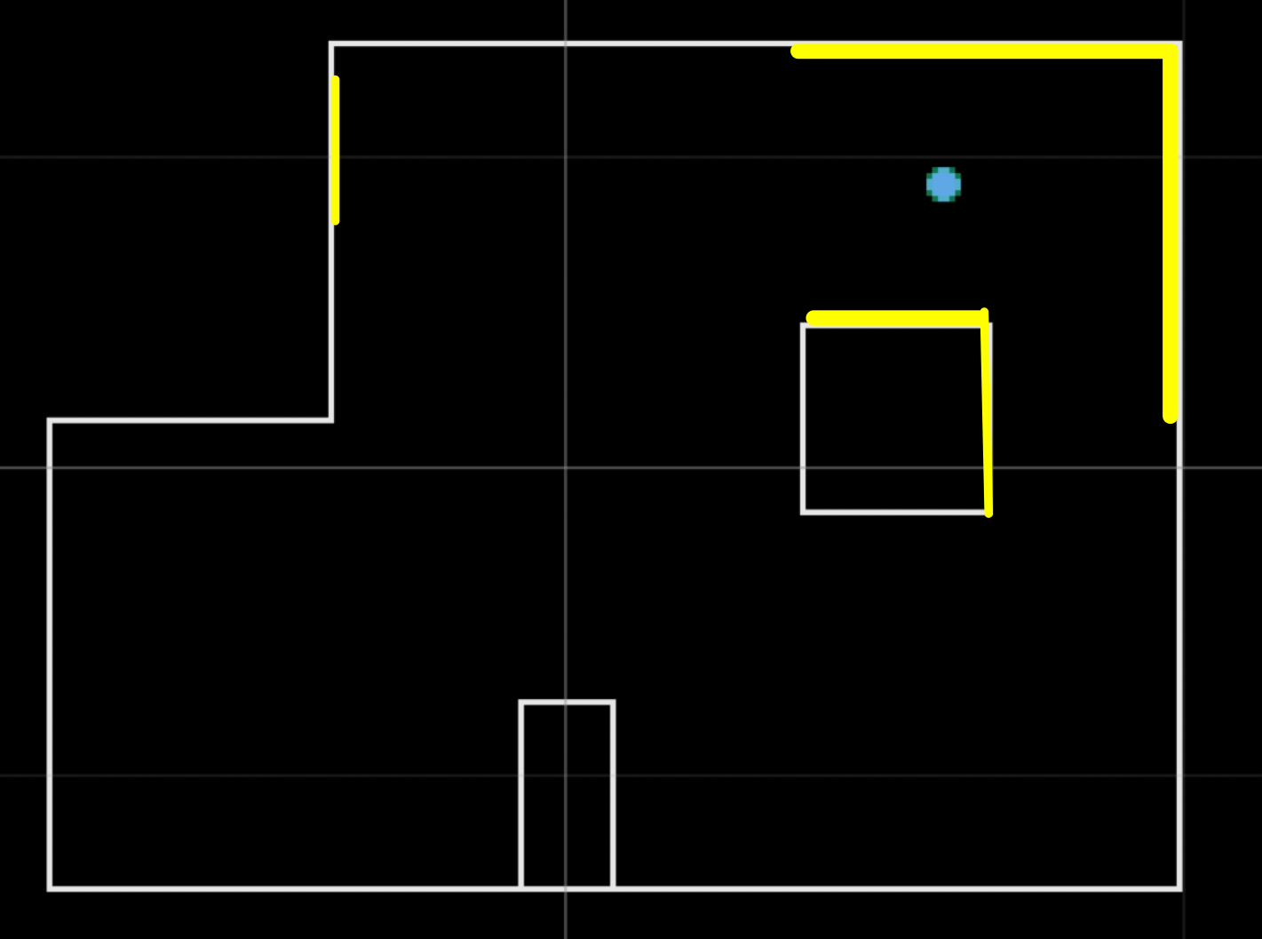
Below are my Belief plots for the locations of interest I mentioned above.
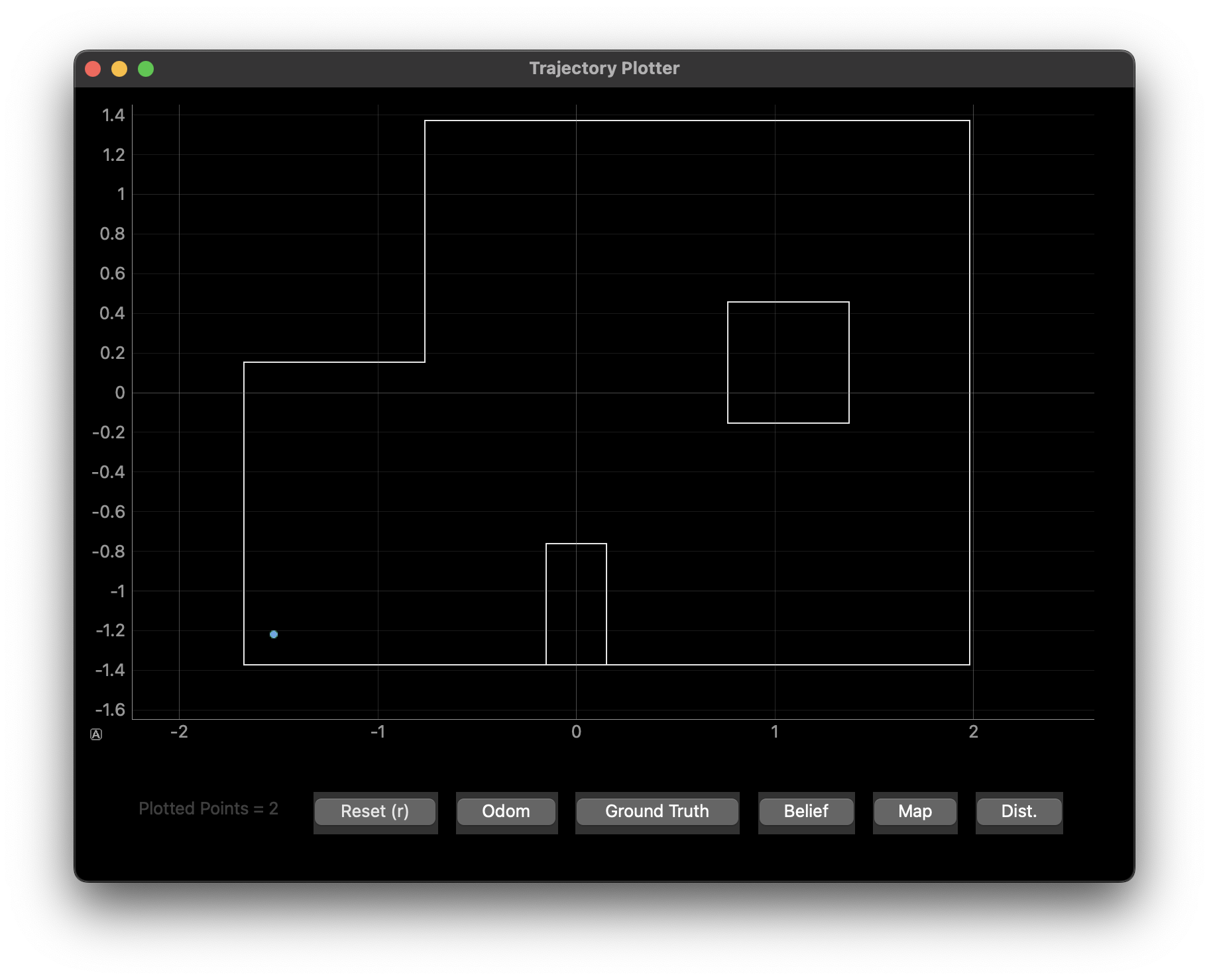
- Location (-3,-2)
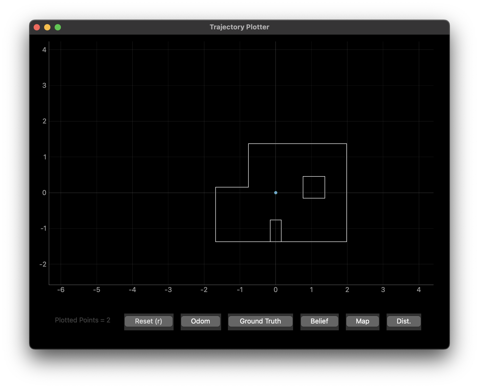
- Location (0,3)
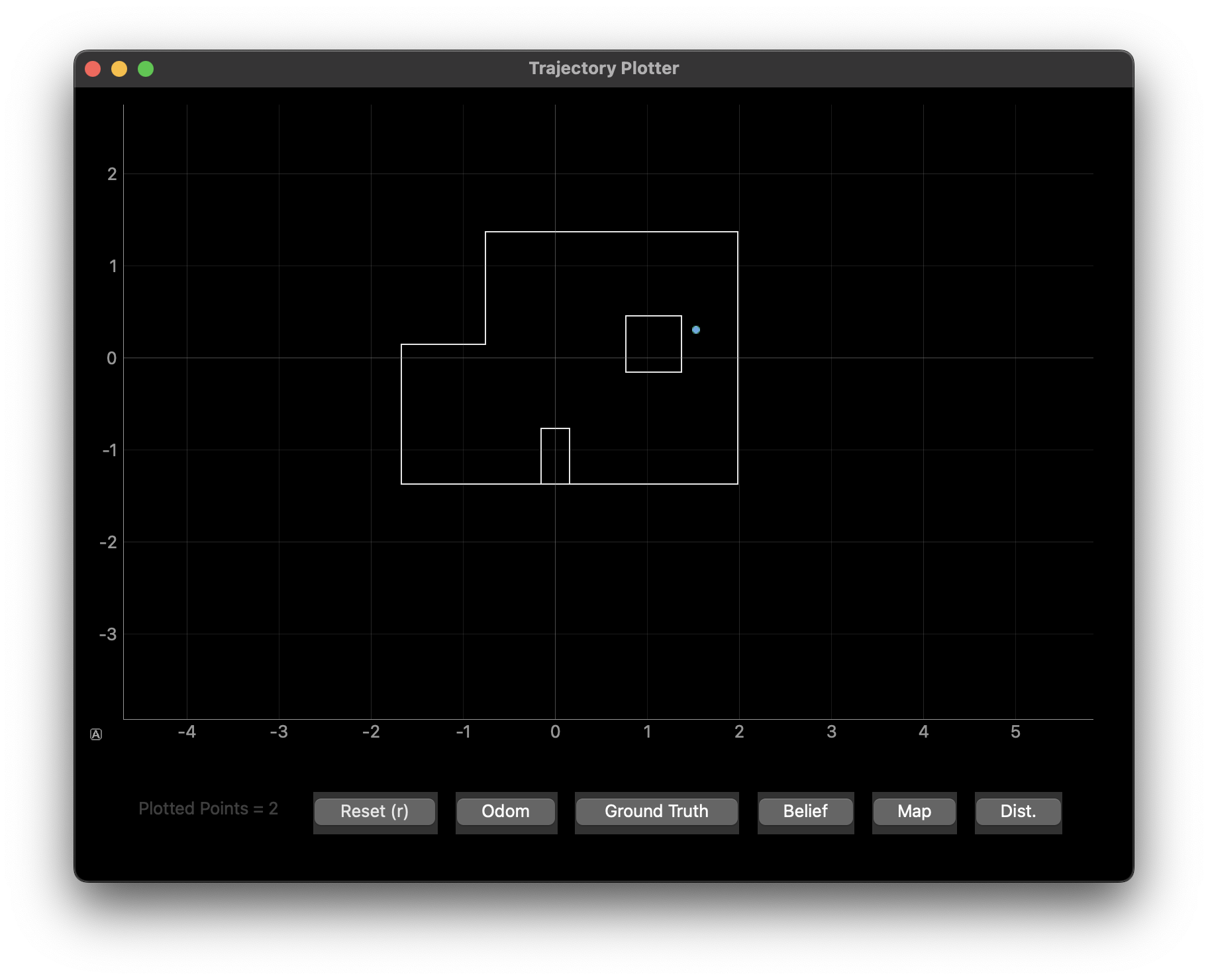
- Location (5,-3)
- Location (5,3)
Discussion
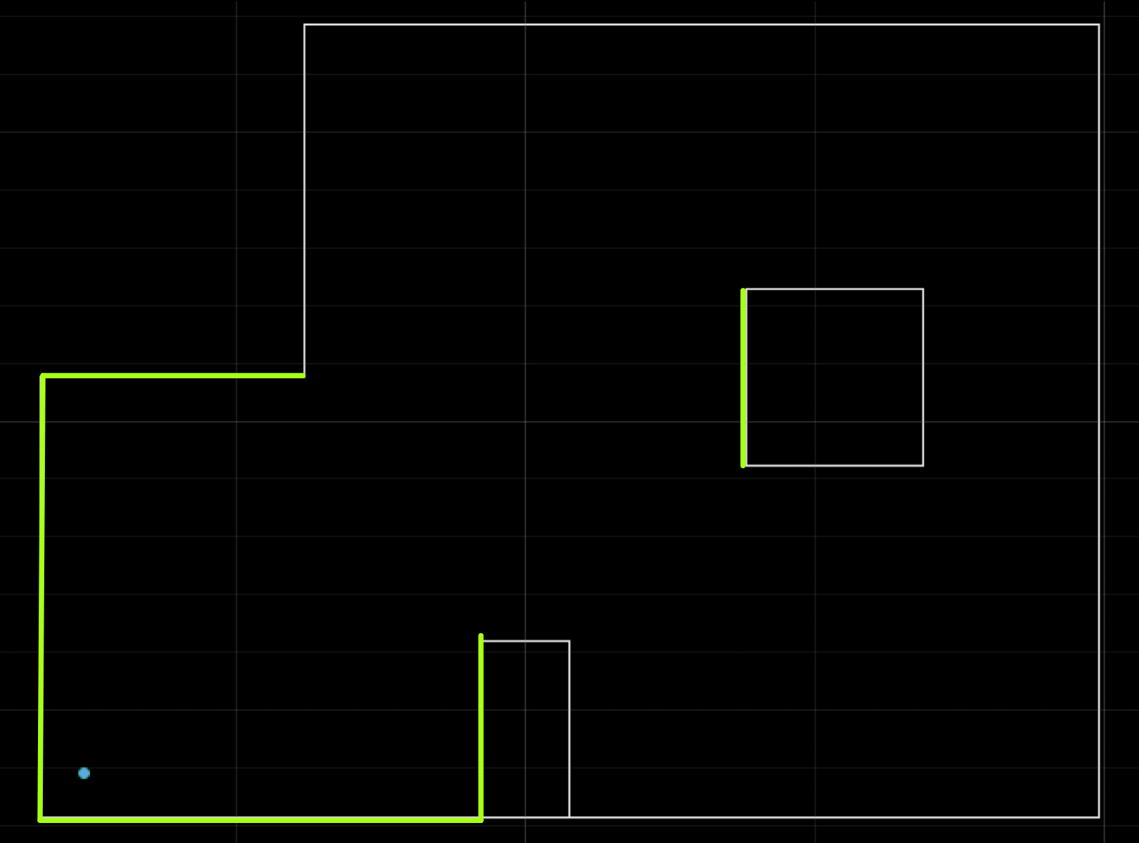
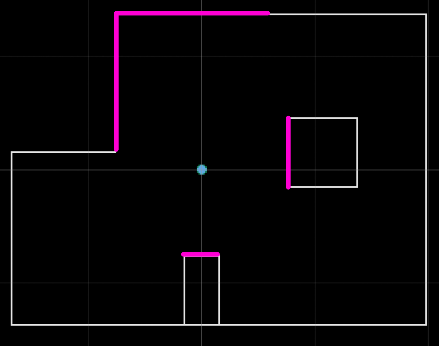
Albeit that my visualized plots are not perfectly at the position where they need to be, the majority of the beliefs seems to demonstrate that it understands the general idea of its surroundings. We can see in particular that there is really only one outlier out of all the plots and that is plot (5,-3). A possible rationale for why this location was not accurately displayed could be because the surroundings at the position (5,-3) shared heavy similarities with other locations such (5,3). Particularly, the symmetry of position (5,-3) is almost identical to (5,3) if the robot is slightly offset and angled differently. See the below two figures for reference.
- Location (5,3)
- Location (5,-3)

- Location (-3,-2)
- Location (0,3)
Takeaway
To conclude, I learned that in the simulated version this lab, we make many assumptions that allow for an almost idealized localization of the robot. However, some of those assumptions are not represented in the physical model and that is represented in the discrepancy in the localization accuracy of the physical robot. Of course, there are improvements we could otherwise do to better our localization model, but this lab made me appreciate the differences apparent in the simulated vs real localization programs