Lab 9: Mapping
Objectives:
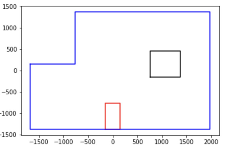
The purpose of this lab is to build up a map of a static room. The map will be used later for localization and navigation tasks. To build the map, the robot is set down in a couple of marked up locations around the lab, and then spun around its axis while measuring its ToF readings. If done successfully the map should end up looking like the plot below.
Materials
- 1 x Fully assembled robot, with Artemis, TOF sensors, and an IMU.
Lab Taks
PID Control
In order to realize the map of the lab environement I leveraged the same methodology used in Lab 6. In that lab I implemented a P(ID) controller using the ToF sensors but in this lab I'll be using the IMU (gyrosocpe) sensor as my reference for the contoroller. As a reminder, the input for system regulation is informed by the following formula:
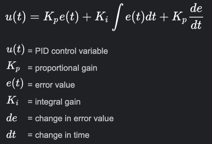
The goal here is to make the robot rotate with an angular velocity (ω) = 15 deg/s. I set the benchmark pwm analog value to be 110. 110 was choosen because that was the lowest pwm value my car could use to execute a smooth turn. Nonetheless, based on the angular speed read from the gyrosocpe, the pwm value would be modified to do accomodate the necessary speed required to maintain a constant ω of 15 deg/s. More concretely, if the measured gyroscope reading is above 15 deg/s the error is positive and will be subtracted from the benchmark of pwm value of 110 and the new result will be the new pwm input in to the motors. Likewise if the car is spinning slower than 15 deg/s the error becomes negative and the pwm value is incremented to an analog value higher than 110. Lastly, if the error is zero, a constant pwm value of 110 will be fed into the motors. See the code snippet below for a high level overview of the algorithm I used for the P(ID) controller.
Map Scan Turn
Visualizing the Map
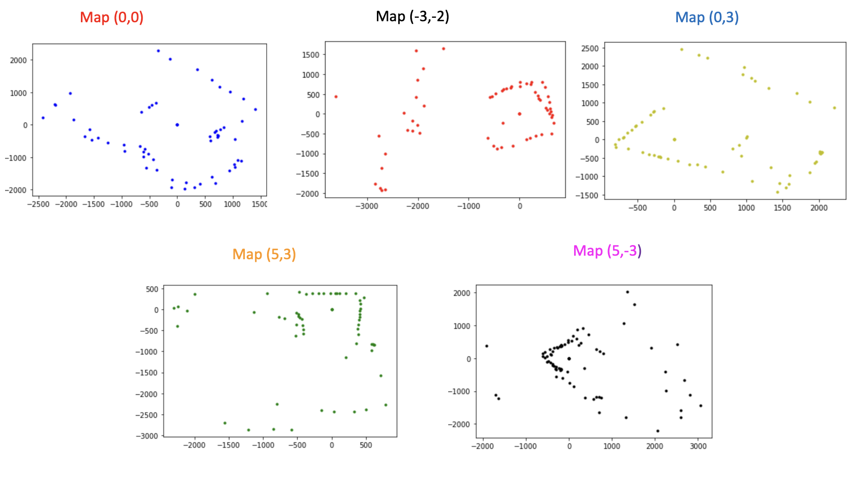
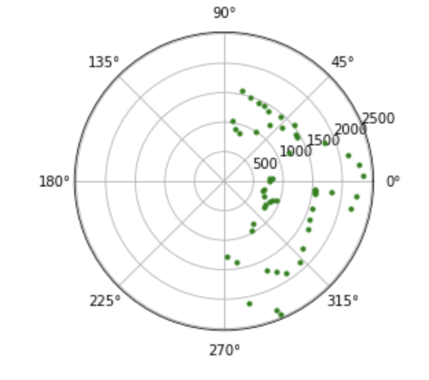
With the program running as intended on the robot, I had the robot send the measured distances of the ToF along with it's associated angle to my computer over bluetooth and I constructed a polar plot with the received data. There were 5 coordinate points of interest within the lab environment: { [0,0],[5,3],[-3,-2],[5,-3],[0,3] }. The idea is that with a scan in each of these locations, we should be to merge each locations individual plot to recreate the map of the lab floor. Shown below is a polar plot of the robot's data based on a scan in each of the aforementioned coordinates.

A few things to note from this plot is that objects that were closer to robot (indidcated by points on the concentric circles closer to the center of the plot) were measured with greater resolution than those that were not. On the polar plot you're likely to see a trend of scattered plots on concentric circles farther from the center because the ToF measurements were noisier at farther distances. I presume that this effects can be attributed to a few things:
- Limitations of the ToF sensor range
- Materials / Color of the bounndaries within the scanned environment (i.e if the wall or wood was black, the ToF light signal might have been absorbed by the dark material which caused a signal loss/ incorrect measurement)
- The rotation rate of the robot car was too fast
Merging the Plots to Create the Map
To create the map, we had to take data we ploted on the polar plot and convert it to a conglomeration of a cartesian based plot of all the points ploted from the 5 different coordinate location. The following formulas was used to convert from polar form to cartesian.
X = ToF_Distance Reading * Cosine (Angle of Car)
Y = ToF_Distance Reading * Sine (Angle of Car)
Cartesian Converion of Polar Plots
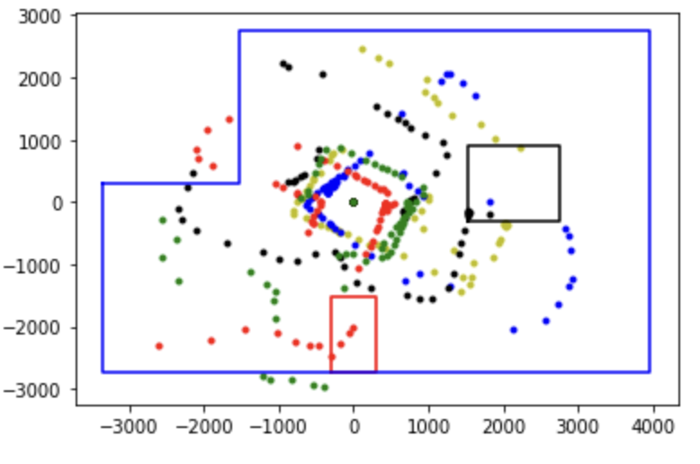
If you observe my polar plots you can see that my scans do not consistently follow the same orientation. When I tried to merge the inidviduals, this inconsistency became emphasized as the merged map came out looking like the figure below.
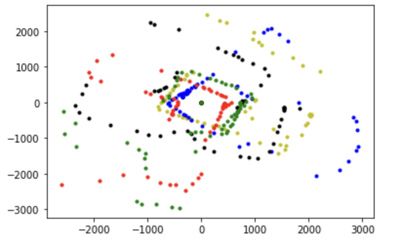
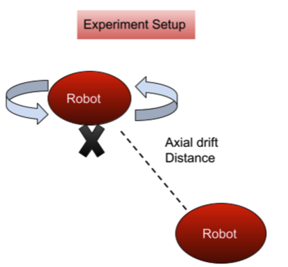
I think this inconsistency in part was due to my variations of the initial orientation of the robot before it started scanning. In addition to this, I also think that it could have also been a result of the axial drift in car's rotation during the scan. Displayed in the figure below is the concept I mean when I say "drift". You'll also notice this motion in the video above when the car is scanning.
To fix this, I took the data points I had and attempted to do the following:
-
I tried to rotate the data points by converting to back from cartesian to polar but this conversion only squeezed all my angles into two quadrants due to aliasing and principal angle selection from the python math.atan() function. Compare the figure below with Map (0,0) from my original polar plot to see what I mean.
- I also tried adding and subtracting to the X, Y coordinates based on where I took the scan fom (i.e making all my coordiantes relative to the 0,0 position) but that didn't work either.
Conclusion: My plot vs Real plot
In light of all I tried, my post processing fixes of the mapping was not successful as my scattered plot vs the real plot (shown above) were not close at all but I learned alot during this lab. I learned how to map, what methods I could use to achieve a better mapping execution and how to do post processing when things go wrong. In the future I would make sure to use the same orientation evdery time when I start scanning and perhaps set my scanning speed to be much lower for better resolution.