Lab 11b: LQR on the Inverted Pendulum on a Cart (sim)
Objective
The purpose of the lab is to become familiar with linear controllers, LQR control and the cost functions to stabilize an inverted pendulum.
Feedback control of an idealized pendulum on a cart system
First, I changed the dimensions of the cart to fit my real life robot, which was 6.5 in by 5.5 by 4.5 in (L X W X H). This adjustment was made in pendulumParam.py. The units in the code were meters, so I convereted accordingly.

I ran the simulator after without a controller and the pendulum was swinging back and forth as expected. Similar to real life, the oscillation died down slowly, which can be seen in the video.
I added a Kr controller and saw that poles -1,-2,-3,-4 were able to stabilize the inverted pendulum. These values were randomly chosen, but the pole had to be in the left hand side of the real/imaginary axis in order to be stable, which is why all the values are negative.

I also used linear quadratic regulator (LQR) built in function in MATLAB to calculate gains. Q is the penalty matrix for the state (z,zdot,theta,thetadot). For Q matrix, I gave small penalty to z and zdot because the inverted pendulum is mainly dependent on theta and thetadot for its position. The penalties for theta and thetadot were given a much higher value. R is another penalty matrix and I decided to test the cart's stability with various values, such as 0.001, 1, and 10. The code for calculating the gain is shown below.
m1 = 0.03;  %Mass of the pendulum [kg]
m2 = .458;  %Mass of the cart [kg]
ell = 1.21; %Length of the rod [m]
g = -9.81;  %Gravity, [m/s^2]
b = 0.78;   %Damping coefficient [Ns]

A = [0.0, 1.0, 0.0, 0.0;...
	0.0, -b/m2, -m1*g/m2, 0.0;...
	0.0, 0.0, 0.0, 1.0;...
	0.0, -b/(m2*ell), -(m1+m2)*g/(m2*ell), 0.0];

B = [0.0;1.0/m2;0.0;1.0/(m2*ell)];

C = [1.0, 0.0, 0.0, 0.0;...
		0.0, 1.0, 0.0, 0.0;...
		0.0, 0.0, 1.0, 0.0;...
		0.0, 0.0, 0.0, 1.0];

Q = [1.0, 0.0, 0.0, 0.0;...
0.0, 1.0, 0.0, 0.0;...
0.0, 0.0, 10.0, 0.0;...
0.0, 0.0, 0.0, 100.0];

R = 0.001;

K = lqr(A,B,Q,R)
I tested the following R penalty values and got the corresponding gain values. It seems that the higher of the penalty, the faster the robot responds to the rod falling. This can be seen in the videos below.
| Case | Penalty (R) | Gain (K) |
|---|---|---|
| 1 | R = 0.001 | K = (-31.6228, -77.4513, 761.5603, 412.6104) |
| 2 | R = 1 | K = (-1.0000, -3.4581, 32.2456, 14.9892) |
| 3 | R = 10 | K = (-0.3162, -2.0436, 18.7336, 7.1975) |
| Case 1 | Case 2 | Case 3 |
|---|---|---|
I tested the limits on what penalty I can give until the robot becomes unstable. With many trials and error, I was able to get an unstable system with Q and R values below.

Feedback control of a non-ideal pendulum on a cart system
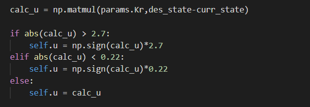
In order to imitate a non-ideal pendulum, I added minimum (deadband) and maximum (saturation) force input on the robot. I calculated the minimum force limit as the friction force that the robot would have to overcome. This was calculated by taking a coefficient of friction of 0.05 and multiplying it with its mass and gravity. The mass was found to be 458 grams from lab 3 and the minimum force was calculated to be 0.22 N. The maximum force was determined by another student (Chris) from his observations during lab 3. The maximum force exertable by the robot is 2.7 N. I implemented these limits using the code below.
I've had a lot of trouble stabilizing the system. I made an adjustments in runSimulation file as suggested on Campuswire. I changed the amplitude and frequency of reference input.

I ran the simulator without adjusting the Q and R values, but as expected it was unstable. I tested with various values and increased R from 0.001 to 10 and it became stable with Q and R values shown below. You can see from the video and the performance graph that the robot has to oscillate often in order to maintain stability

