Lab 8: Grid Localization using Bayes Filter
Objective
The purpose of this lab is to implement grid localization using Bayes Filter on the simulator.
Procedure
For localization, I implemented using the Bayesian filter code below and attached here. The bayesian filter mainly consists of the predict and update step. The predict step requires the likelihood that the "robot" is in a certain place given the previous location and the controls, which can be calculated in odom_motion_model and compute_control. The update step is updating the new position given the sensor measurements and the prediction, which is calculated in sensor_model and update_step.
def compute_control(cur_pose, prev_pose):
	""" Given the current and previous odometry poses, this function extracts
	the control information based on the odometry motion model.

	Args:
		cur_pose  ([Pose]): Current Pose
		prev_pose ([Pose]): Previous Pose

	Returns:
		[delta_rot_1]: Rotation 1  (degrees)
		[delta_trans]: Translation (meters)
		[delta_rot_2]: Rotation 2  (degrees)
	"""

	# calculating translation
	delta_x = cur_pose[0] - prev_pose[0]  #change in position in the x direction
	delta_y = cur_pose[1] - prev_pose[1]  #change in position in the y direction
	delta_trans =  math.sqrt(delta_x**2 + delta_y**2)  #distance between current pose and previous pose

	# calculating rotation 1 and 2 and convert to degrees and normalizing the angle

	delta_rot_1 = loc.mapper.normalize_angle((math.atan2(delta_y,delta_x)*180/np.pi) - cur_pose[2])
	delta_rot_2 = loc.mapper.normalize_angle(cur_pose[2] - prev_pose[2] - delta_rot_1)

	return delta_rot_1, delta_trans, delta_rot_2

# In world coordinates
def odom_motion_model(cur_pose, prev_pose, u):
	""" Odometry Motion Model

	Args:
		cur_pose  ([Pose]): Current Pose
		prev_pose ([Pose]): Previous Pose
		(rot1, trans, rot2) (float, float, float): A tuple with control data in the format
													format (rot1, trans, rot2) with units (degrees, meters, degrees)


	Returns:
		prob [float]: Probability p(x'|x, u)
	"""

	#get controls given the previous and current pose
	odom_motion = compute_control(cur_pose,prev_pose)

	#comput the difference between the calculated controls and actual controls
	x1 = u[0] - odom_motion[0]   #error in rot1
	x2 = u[1] - odom_motion[1]   #error in trans
	x3 = u[2] - odom_motion[2]   #error in rot2

	rot1_prob = loc.gaussian(x1,0,loc.odom_rot_sigma)      #finding the probability that the measurement is accurate
	trans_prob = loc.gaussian(x2,0,loc.odom_trans_sigma)
	rot2_prob = loc.gaussian(x3,0,loc.odom_rot_sigma)

	prob = rot1_prob*trans_prob*rot2_prob                  #multiplying all the probabilities assuming they are independent
	return prob


def prediction_step(cur_odom, prev_odom):
	""" Prediction step of the Bayes Filter.
	Update the probabilities in loc.bel_bar based on loc.bel from the previous time step and the odometry motion model.

	Args:
		cur_odom  ([Pose]): Current Pose
		prev_odom ([Pose]): Previous Pose
	"""

	u = compute_control(cur_odom, prev_odom)                          #calculating controls given the final and previous positions
	for prev_x in range(mapper.MAX_CELLS_X):                          #iterate through previous x
		for prev_y in range(mapper.MAX_CELLS_Y):                      #iterate through previous y
			for prev_theta in range(mapper.MAX_CELLS_A):              #iterate through previous theta
				if (loc.bel[prev_x][prev_y][prev_theta]>0.0001):
					for cur_x in range(mapper.MAX_CELLS_X):                                       #iterate through current x
						for cur_y in range(mapper.MAX_CELLS_Y):                                   #iterate through current y
							for cur_theta in range(mapper.MAX_CELLS_A):                           #iterate through current theta
								curr_pose = mapper.from_map(cur_x,cur_y,cur_theta)      #getting the current pose from mapper
								prev_pose = mapper.from_map(prev_x,prev_y,prev_theta)   #getting the previous pose from mapper
								#use the given grid pose make prediction for each grid
								loc.bel_bar[cur_x][cur_y][cur_theta] += odom_motion_model(curr_pose,prev_pose, u) * loc.bel[prev_x][prev_y][prev_theta]
	loc.bel_bar = loc.bel_bar/np.sum(loc.bel_bar)

def sensor_model(zt,xt):
	""" This is the equivalent of p(z|x).

	Args:
		zt ([ndarray]): A 1D array consisting of the measurements made in rotation loop
		xt are cell numbers (x,y,theta)
	Returns:
		[ndarray]: Returns a 1D array of size 18 (=loc.OBS_PER_CELL) with the likelihood of each individual measurements
	"""
	#initializing prob_array
	(a,b,c) = xt
	prob_array = np.zeros(mapper.OBS_PER_CELL)
	#iterate through all the measurements
	for i in range(mapper.OBS_PER_CELL):
		#find the probability of measurement given data
		prob_array[i] = loc.gaussian(zt[i],loc.mapper.get_views(a,b,c)[i],loc.sensor_sigma)

	return prob_array

def update_step():
	""" Update step of the Bayes Filter.
	Update the probabilities in loc.bel based on loc.bel_bar and the sensor model.

	Args:
		zt ([ndarray]): A 1D array consisting of the measurements made in rotation loop

	"""

	for x in range(mapper.MAX_CELLS_X):                                       #iterate through current x
		for y in range(mapper.MAX_CELLS_Y):                                   #iterate through current y
			for a in range(mapper.MAX_CELLS_A):
				loc.bel[x][y][a] = np.prod(sensor_model(loc.obs_range_data,(x,y,a)))*loc.bel_bar[x][y][a]

	loc.bel = loc.bel / np.sum(loc.bel)
I started up the simulator and plotter to test the localization. First, I tested the trajectory using only odometry. In the graph below, green line indicates the global truth pose and the blue indicated odometry pose. The odometry can sometimes capture the overall trajectory, but is inaccurate in terms of the robot's location. In the video, you can see that the location is completely off the boundary limits.

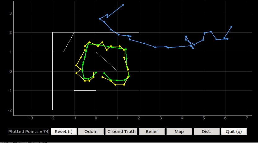
After, I tested the same trajectory with the Bayes filter and got the trajectory below. The green is truth pose, blue is odometry and yellow is belief from Bayesian filter. As seen in the image, the trajectory is much more accurate than odometry because it takes in to consideration sensor measurements that helps estimate its location. The process can be seen in the video. The filter takes a while to process all the probabilities and sensor measurements, so it took about 11 mins total to make its trip around the map.