Lab 7(a): Grid Localization using Bayes Filter
Objective
The purpose of this lab is to write a skeleton Bayes Filter algorithm that will be implemented in the next lab.
# In world coordinates
def compute_control(cur_pose, prev_pose):
    """ Given the current and previous odometry poses, this function extracts
    the control information based on the odometry motion model.

    Args:
        cur_pose  ([Pose]): Current Pose [x y theta]
        prev_pose ([Pose]): Previous Pose [x y theta]

    Returns:
        [delta_rot_1]: Rotation 1  (degrees)
        [delta_trans]: Translation (meters)
        [delta_rot_2]: Rotation 2  (degrees)
    """

    # calculating translation
    delta_x = cur_pose[0] - prev_pose[0]
    delta_y = cur_pose[1] - prev_pose[1]
    delta_trans =  np.sqrt(delta_x**2 + delta_y**2)

    # calculating rotation 1 and 2
    delta_rot_1 = np.arctan2(delta_y,delta_x) - cur_pose[2]
    delta_rot_2 = cur_pose[2] - prev_pose[2] - delta_rot_1

    return delta_rot_1, delta_trans, delta_rot_2

# In world coordinates
def odom_motion_model(cur_pose, prev_pose, u):
    """ Odometry Motion Model

    Args:
        cur_pose  ([Pose]): Current Pose
        prev_pose ([Pose]): Previous Pose
        (rot1, trans, rot2) (float, float, float): A tuple with control data in the format
                                                   format (rot1, trans, rot2) with units (degrees, meters, degrees)


    Returns:
        prob [float]: Probability p(x'|x, u)
    """

    odom_motion = compute_control(cur_pose,prev_pose)
    rot1_odom = odom_motion[0]
    trans_odom = odom_motion[1]
    rot2_odom = odom_motion[2]
    rot1_rel = u[0]
    trans_rel = u[1]
    rot2_rel = u[2]

    x1 = rot1_odom - rot1_rel  #error in rot1
    x2 = rot2_odom - trans_rel #error in trans
    x3 = rot3_odom - rot2_rel  #error in rot2
    sigma1 = odom_rot_sigma    #standard deviation for rot1
    sigma2 = odom_trans_sigma  #standard deviation for trans
    sigma3 = odom_rot_sigma    #standard deviation for rot2

    rot1_prob = gaussian(x1,0,sigma1)
    trans_prob = gaussian(x2,0,sigma2)
    rot2_prob = gaussian(x3,0,sigma3)

    prob = rot1_prob*trans_prob*rot2_prob

    return prob

def prediction_step(cur_odom, prev_odom):
    """ Prediction step of the Bayes Filter.
    Update the probabilities in loc.bel_bar based on loc.bel from the previous time step and the odometry motion model.

    Args:
        cur_odom  ([Pose]): Current Pose
        prev_odom ([Pose]): Previous Pose
    """
    u = compute_control(cur_odom, prev_odom)
    for cur_x in range(MAX_CELLS_X-1):                          #iterate through current x
        for cur_y in range(MAX_CELLS_Y-1):                      #iterate through current y
            for cur_theta in range(MAX_CELLS_A-1):              #iterate through current theta
                for z in range(obs_views[x,y,theta,:])      #iterate through obs_views to add all the 18 x and y positions inside that grid
                    [xpos,ypos] += obs_views[cur_x,cur_y,cur_theta,z]
                grid_pose = [xpos,ypos]/length(obs_views[x,y,theta,:]) #take the mean of that summed x and y position to find the position of that grid

                for prev_x in range(MAX_CELLS_X-1):                          #iterate through previous x
                    for prev_y in range(MAX_CELLS_Y-1):                      #iterate through previous y
                        for prev_theta in range(MAX_CELLS_A-1):              #iterate through previous theta
                            for z2 in range(obs_views[x,y,theta,:])           #iterate through obs_views to add all the 18 x and y positions inside that grid
                                [xpos2,ypos2] += obs_views[x,y,theta,z]
                            prev_pose = [xpos2,ypos2]/length(obs_views[prev_x,prev_y,prev_theta,:]) #take the mean of that summed x and y position to find the position of that grid
                            loc.bel_bar += odom_motion_model(grid_pose,prev_pose, u) * loc.bel[cur_x,cur_y,cur_theta]#use the given grid pose make prediction for each grid


def sensor_model(zt,xt):
    """ This is the equivalent of p(z|x).


    Args:
        zt ([ndarray]): A 1D array consisting of the measurements made in rotation loop
        xt: current state

    Returns:
        [ndarray]: Returns a 1D array of size 18 (=loc.OBS_PER_CELL) with the likelihood of each individual measurements
    """

    for i in range(length(zt)): #iterate through all the measurements
        error = zt-xt
        prob_array[i] = gaussian(error,0,sigma) #find the probability of measurement given data

    return prob_array

def update_step(zt,xt):
    """ Update step of the Bayes Filter.
    Update the probabilities in loc.bel based on loc.bel_bar and the sensor model.
    """
    normalization = 1/(sum of all the bel_bar probabilities)
    loc.bel = normalization*sensor_model(zt,,xt)*loc.bel_bar
Lab 7(b): Mapping
Objective
Purpose of this lab is to build a map of my room and to perform PID from last lab.
Procedure
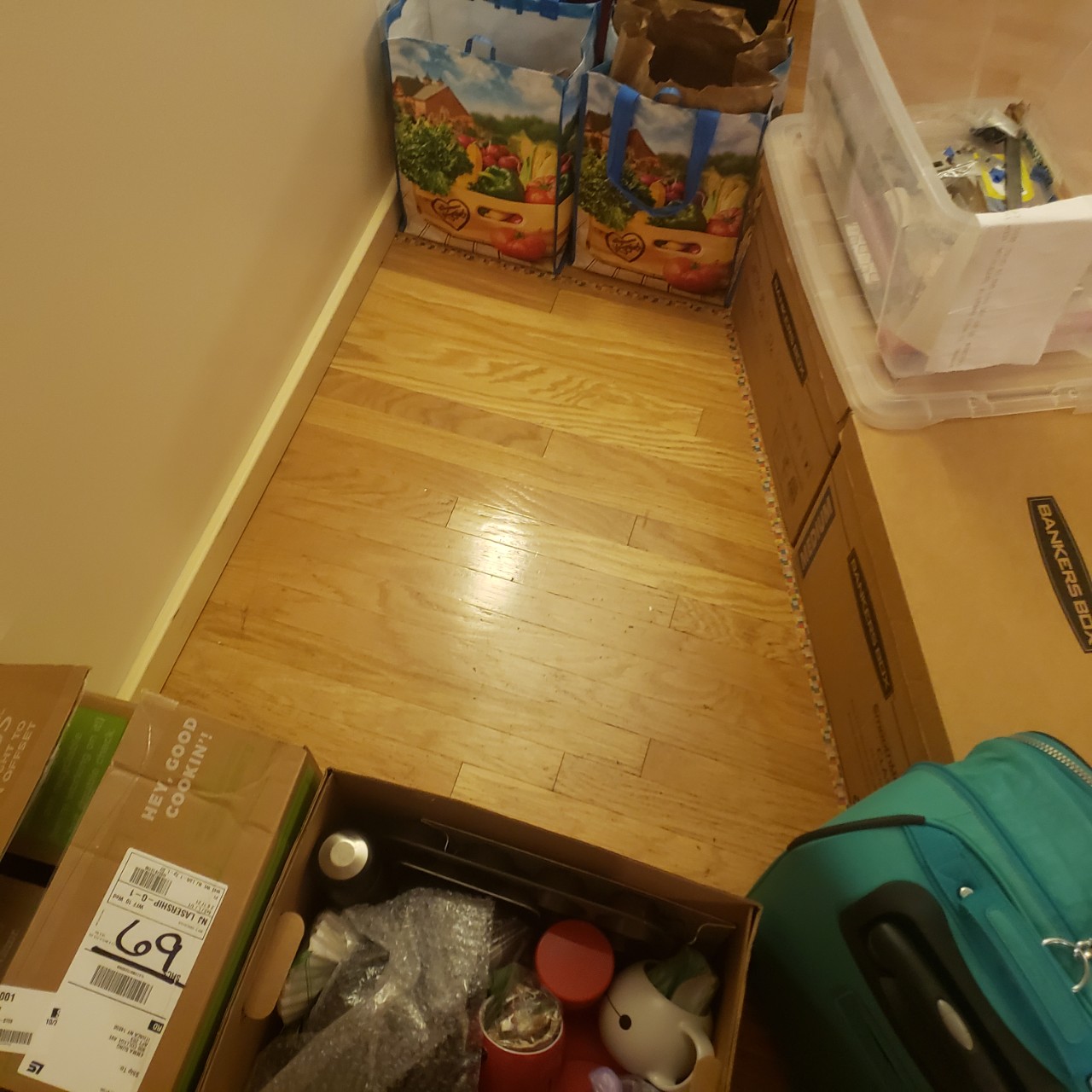
- I allocated a space in my apartment for the robot to roam in.
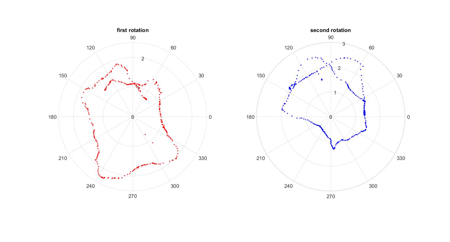
- I checked if my robot could do a full rotation. I had some difficulty with PID last week, but I was able to manually pick motor speeds that allowed the robot to rotate. My sensor data had significant noise, but this is not unexpected since I was having difficulty with PID controller. I gathered the data and plotted the data points in the polar coordinates in MATLAB.
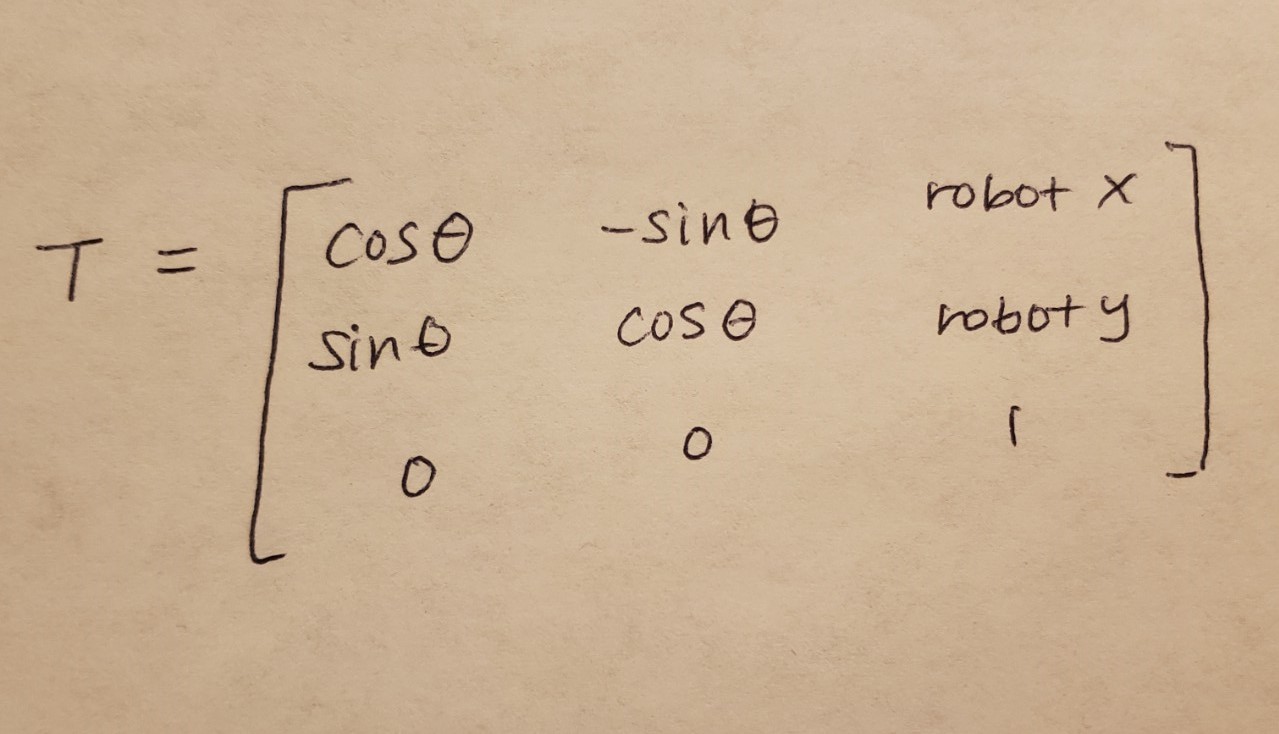
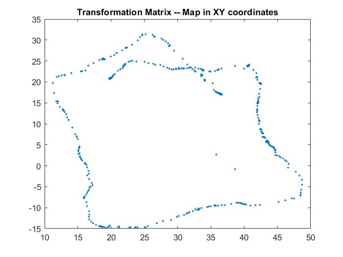
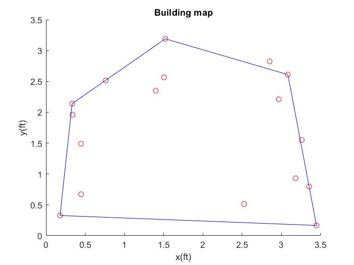
- I used transformation matrix to convert the data from polar coordinates to cartesian coordinates using the transformation matrix. Using the equation, I was able to get the xy coordinates as shown below.
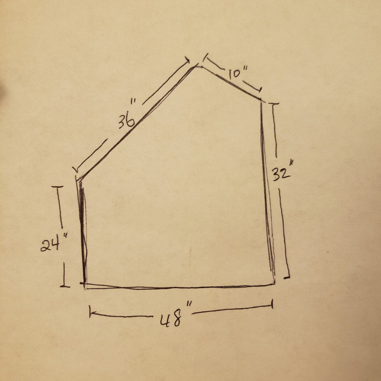
- I collected data points through line scans and used known positions and orientation of robot. This allowed the transformation matrix to convert the data to cartesian coordinates with origin matched up with the left corner of the map. I drew what the map is supposed to look like with measurements in inches and plotted the collected data from line scans. The line scan did a good job capturing the features of the map, but may had some difficulty getting accurate dimensions. This may be due to the noise of the data.
- I saved the points from the scatter plot above and plotted it in the simulator using plotter.py.
